In the following calculations:
We’ll exploit the symmetry of the Schwarzschild geometry to ignore one space coordinate: θ, defined as the angle from some direction chosen as the coordinate “pole”, will be taken to be fixed at π/2, i.e. we’ll work entirely within the “equatorial plane” of the coordinate system. The motion of any single particle can be analysed in the remaining three spacetime coordinates, simply by choosing the equatorial plane to coincide with the plane of the particle’s orbit.
With this restriction, the Schwarzschild metric gives the dot product between two arbitrary 4-vectors v and w as:
| g(v, w) | = | –(1–2M/r) vt wt + 1/(1–2M/r) vr wr + (r2) vφ wφ | (1a) |
We’ll also make use of the flat-space polar-coordinates Lorentzian metric, far from the hole:
| g(v, w) | = | – vt wt + vr wr + (r2) vφ wφ | (1b) |
Replacing M/r with u in (1a) gives:
| g(v, w) | = | –(1–2u) vt wt + 1/(1–2u) vr wr + (M/u)2 vφ wφ | (2) |
In all of the above, vt, vr, vφ etc. are the components of the vectors in the (non-orthonormal) basis {∂t, ∂r, ∂φ}, so:
| v | = | vt ∂t + vr ∂r + vφ ∂φ |
| w | = | wt ∂t + wr ∂r + wφ ∂φ |
An observer with constant r and φ (outside the hole) has a 4-velocity:
| w | = | 1/√(1–2u) ∂t | (3, outside) |
while an observer with constant t and φ (inside the hole) has a 4-velocity:
| w | = | –√(2u–1) ∂r | (4, inside) |
[As a check, both of these yield g(w, w) = –1, as every 4-velocity must, and they both point into the future: (3) obviously, and (4) because r is now timelike, having a negative component in the metric, and decreasing r is the future.]
The energy an observer with 4-velocity w measures for a photon with energy-momentum 4-vector p is:
| E | = | –g(p, w) | (5) |
This is just projecting out the timelike component of the energy-momentum vector, in the observer’s rest frame.
The simplest method for analysing geodesics near a black hole is to use Killing’s equation (see Gravitation by Misner, Thorne and Wheeler, sections 25.2, 25.3). The vector fields ∂t and ∂φ are Killing vectors, because the Schwarzschild geometry is static, and axially symmetric. So along any geodesic, there are two conserved quantities:
| g(p, ∂t) | = | K1 | (6a) |
| g(p, ∂φ) | = | K2 | (6b) |
To put physically meaningful values to these constants, follow the geodesic back to infinity. Far from the hole, the photon is essentially travelling along the straight line (in Cartesian coordinates):
| y | = | bM |
where b is the impact parameter divided by M. Assume it’s at large +ve x, heading towards the x-axis; then its energy-momentum 4-vector is:
| p | = | E∞ ∂t – E∞ ∂x |
Converting to polar coordinates:
| ∂x | = | (dr/dx)∂r + (dφ/dx)∂φ | |
| = | (x/r) ∂r – (y/r2) ∂φ | ||
| p | = | E∞ ∂t – E∞ (x/r) ∂r + E∞ (y/r2) ∂φ |
[As a check: g(p, p) = 0 for the flat Lorentzian metric (1b), its spatial part points in the right direction (-ve x, or -ve r and +ve φ), its time part is future-directed, and it gives the right energy in Eqn (5), putting w=∂t and again using the flat metric (1b).]
Substituting this into Eqn (6a) – still using the flat metric – gives:
| K1 | = | –E∞ | |
| g(p, ∂t) | = | –E∞ | (7a) |
Substituting into (6b):
| K2 | = | g(p, ∂φ) | |
| = | y E∞ | ||
| = | bM E∞ | ||
| g(p, ∂φ) | = | bM E∞ | (7b) |
[Eqns (7a) and (7b) are statements of conservation of energy and conservation of angular momentum.]
While we’re at it, it’s useful to work out the third analogous expression:
| g(p, ∂r) | = | F(u) | |
| = | ??? | (7c) |
even though this quantity isn’t conserved. Forget about being at infinity now, and in all generality write p in terms of the basis vectors:
| p | = | pt ∂t + pr ∂r + pφ ∂φ | (7d) |
Applying Eqn (7a) to this yields:
| –E∞ | = | pt g(∂t, ∂t) | |
| = | – pt (1–2u) | ||
| pt | = | E∞ / (1–2u) |
Applying Eqn (7b) yields:
| bM E∞ | = | pφ g(∂φ, ∂φ) | |
| = | pφ (M/u)2 | ||
| pφ | = | bM E∞ (u/M)2 |
And applying Eqn (7c) yields:
| F(u) | = | pr g(∂r, ∂r) | |
| = | pr / (1–2u) | ||
| pr | = | F(u) (1–2u) |
Substituting all these coefficients back into (7d), and then using the fact that p must be a null vector, so g(p, p) = 0 in the metric of Eqn (2):
| 0 | = | –(1–2u) [pt]2 + 1/(1–2u) [pr]2 + (M/u)2 [pφ]2 | |
| 0 | = | –(E∞)2 / (1–2u) + F(u)2 (1–2u) + (bM E∞)2 (u/M)2 |
| F(u)2 | = | E∞2 [1 – b2u2(1–2u)] / (1–2u)2 |
Depending on whether we’re looking at the photon ascending or descending, this gives:
| g(p, ∂r) | = | F(u) | |
| = | ± E∞ √[1 – b2u2(1–2u)] / (1–2u) |
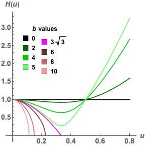
The expression √[1 – b2u2(1–2u)] turns up so often in these calculations that it’s worth defining an abbreviation for it:
| H(u) | = | √[1 – b2u2(1–2u)] | |
| = | √[1 + b2u2(2u–1)] |
which gives a more compact formula:
| g(p, ∂r) | = | F(u) | |
| = | ± E∞ H(u) / (1–2u) | (7e) |
[As a check, put b = 3√3, the impact parameter for marginal capture (see Misner, Thorne and Wheeler, section 25.6). Then the closest approach should occur at r = 3M, or u = 1/3. Substituting these values into Eqn (7e) gives:
| g(p, ∂r) | = | ± E∞ √[1 – 27 (1/9) (1/3)] / (1/3) | |
| = | 0 |
as expected.]
|
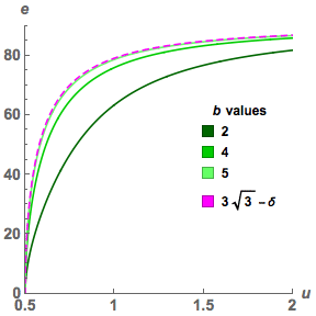
H(u) vs. u, for various impact parameters. Geodesics with impact parameters less than 3√3 end up in the hole, so H(u) never touches zero. Geodesics with larger impact parameters reach their closest approach (highest u) when H(u) = 0. |
For an observer outside the hole with constant r and φ, Eqn (3) gives:
| w | = | 1/√(1–2u) ∂t |
and Eqns (5) and (7a) give an observed energy for the photon of:
| E | = | –g(p, (1/√(1–2u) ∂t) | |
| = | E∞ / √(1–2u) | ||
| E/E∞ | = | 1/√(1–2u) | (8, outside) |
This is the uniform blue shift outside the hole. [Misner, Thorne and Wheeler’s Eqn (25.26) says essentially the same thing, though the notation is different, and they assume an observer at infinity receiving a photon emitted near the hole.]
For an observer inside the hole with constant t and φ, Eqn (4) gives:
| w | = | –√(2u–1) ∂r |
Eqn (5) gives an observed energy for the photon of:
| E | = | –g(p, –√(2u–1) ∂r) | |
| = | √(2u–1) g(p, ∂r) |
and then substituting from Eqn (7e) – choosing the minus sign, because inside the hole the photon must be descending – gives:
| E | = | – E∞ √(2u–1) H(u) / (1–2u) | |
| E/E∞ | = | √[(1 + b2u2(2u–1)) / (2u–1)] |
which simplifies to:
| E/E∞ | = | √[b2u2 + 1/(2u–1)] | (9, inside) |
So for light from the zenith,
| E/E∞ | = | 1 / √(2u–1) |
To convert between b, and angle from the zenith e, it will be shown later that for stationary observers:
| sin(e) | = | b u √(1–2u) | (10a, outside) |
| tan(e) | = | b u √(2u–1) | (10b, inside) |
which gives:
| E/E∞ | = | √[(1+tan2(e))/(2u–1)] |
which simplifies to:
| E/E∞ | = | 1/[√(2u–1) cos(e)] | (11, inside) |
Suppose an observer with rest-mass m free-falls radially into the hole, and suppose their 4-velocity at any position is given by:
| w | = | wt ∂t + wr ∂r |
Then their momentum 4-vector is just:
| p | = | m w | |
| = | m wt ∂t + m wr ∂r |
Equation (6a) applies just as well to an object with rest mass, so:
| g(p, ∂t) | = | m wt g(∂t, ∂t) | |
| = | – m wt (1–2u) | ||
| = | K1 | (12) |
is a constant of motion. If the observer starts from rest at u = u0, then from Eqn (3):
| wt | = | 1/√(1–2u0) |
at u = u0, so:
| K1 | = | – m √(1–2u0) |
and hence:
| g(p, ∂t) | = | – m wt (1–2u) | |
| = | – m √(1–2u0) | ||
| wt | = | √(1–2u0) / (1–2u) | (13) |
But g(w, w) = –1, for any object’s 4-velocity, so we can find wr as well by solving:
| –1 | = | –(1–2u) (1–2u0)/(1–2u)2 + (wr)2 / (1–2u) | |
| wr | = | –√[2(u–u0)] | (14) |
Together, this gives the 4-velocity of the free-falling observer at any u:
| w | = | [√(1–2u0) / (1–2u)] ∂t – √[2(u–u0)] ∂r | (15) |
[As a check, put u=u0 for the start of the fall, and this agrees with Eqn (3).]
Applying Eqn (5) to this, and the photon’s 4-momentum, gives:
| E | = | –g(p, w) | |
| = | – [√(1–2u0) / (1–2u)] g(p,∂t) + √[2(u–u0)] g(p, ∂r) |
Substituting from (7a) and (7e) gives:
| E | = | E∞ {√(1–2u0) / (1–2u) ± √[2(u–u0)] H(u) / (1–2u)} | |
| E/E∞ | = | {√(1–2u0) ± √[2(u–u0)] H(u)} / (1 – 2u) | (16, u > u0) |
[As a check, put u=u0, and this reduces to Eqn (8).]
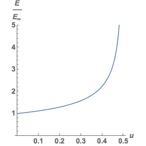
For a specific example, put u0 = 0 (free fall from infinity), and this becomes:
| E/E∞ | = | [1 ± √(2u) H(u)] / (1 – 2u) | (17, anywhere) |
In Eqns (16) and (17), the plus sign is for photons ascending from their closest approach to the hole after failing to be captured, and the minus sign is for descending photons.
 |
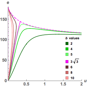
Red/blue shifts, for an observer free-falling radially into the hole from rest at infinity. (Double-valued curves are for ascending/descending photons.) |
To find the angle from the zenith, e, that an observer measures for a photon with a given impact parameter, b, project out the part of the photon’s energy-momentum 4-vector that the observer considers to lie purely in a spatial direction, then find the angle that this vector makes with the same projection for a “reference” photon with impact parameter zero, which comes directly from the zenith.
The angle between these vectors is found with the usual cosine law, using the Schwarzschild metric, Eqn (2), for the dot product:
| cos(e) | = | g(psp,pref) / √[g(psp,psp) g(pref,pref)] |
Because a photon’s energy-momentum 4-vector is a null vector, the length of its spatial part (according to a given observer) must be equal to the length of its timelike part, according to the same observer. And the length of an energy-momentum 4-vector’s timelike part is just its energy, which we’ve already calculated when determining red- and blueshifts for various observers.
So, the simplest way for us to find the angle is by converting the above equation to:
| cos(e) | = | g(psp,pref) / [Eb Eref] | (18) |
where Eb and Eref are the energies the observer in question measures for a photon with impact parameter b, and impact parameter zero.
Gathering together the components of the photon’s energy-momentum 4-vector, previously calculated in deriving Eqn (7e):
| pt | = | E∞ / (1–2u) | (19a) |
| pφ | = | b E∞ u2/M | (19b) |
| pr | = | ± E∞ H(u) | (19c) |
For a stationary observer outside the hole, r and φ are purely spatial coordinates, so the spatial projections for an arbitrary and reference photon are:
| psp | = | ± E∞ H(u) ∂r + b E∞ u2/M ∂φ | |
| pref | = | – E∞ ∂r |
Eqn (18), with energies substituted from Eqn (8), yields:
| cos(e) | = | ± [E∞2 H(u) / (1–2u)] / [E∞2 / (1–2u)] | |
| = | ±H(u) |
Here, the plus sign is for descending photons (which make an acute angle with the zenith), and the minus sign is for ascending photons. This can be rewritten in the form already given in Eqn (10a):
| sin(e) | = | b u √(1–2u) | (20a, outside) |
 |
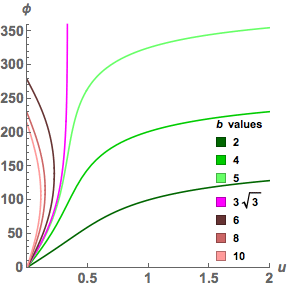
The angle from the zenith a stationary observer outside the hole measures for photons with various impact parameters. The shrinking envelope reflects the gradual shrinking of the sky, as the disk of the hole engulfs it. (Double-valued curves are for ascending/descending photons.) |
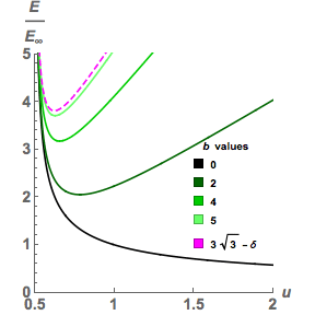
For a stationary observer inside the hole (stationary in the sense that the Schwarzschild t coordinate, which is now spacelike, is constant), t and φ are the purely spatial coordinates, so the spatial projections become:
| psp | = | E∞ / (1–2u) ∂t + b E∞ u2/M ∂φ | |
| pref | = | E∞ / (1–2u) ∂t |
Eqn (18), with energies substituted from Eqn (9), yields:
| cos(e) | = | [E∞2 / (2u–1)] / [E∞2 √[b2u2 + 1/(2u–1)] √[1/(2u–1)]] | |
| = | 1 / H(u) |
This can be rewritten in the form already given in Eqn (10b):
| tan(e) | = | b u √(2u–1) | (20b, inside) |
 |
The angle from the zenith a stationary (t=constant) observer inside the hole measures for photons with various impact parameters. |
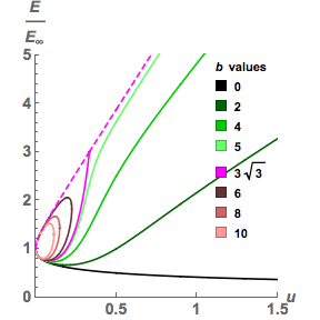
For a radially free-falling observer, φ remains a purely spatial coordinate, but the other spatial direction will lie somewhere in the plane between ∂r and ∂t, orthogonal to the observer’s 4-velocity, already calculated as Eqn (15):
| w | = | [√(1–2u0) / (1–2u)] ∂t – √[2(u–u0)] ∂r | (15) |
The calculation can be carried through for any value of u0, but the easiest case is free-fall from infinity (u0=0). The observer’s 4-velocity then becomes:
| w | = | 1/(1–2u) ∂t – √(2u) ∂r |
and the energy of the photon with impact parameter b is given by Eqn (17):
| Eb/E∞ | = | [1 ± √(2u) H(u)] / (1 – 2u) |
The spatial part of the photon’s energy-momentum 4-vector can be found by subtracting out Eb w:
| psp | = | E∞/(1–2u) ∂t ± E∞ H(u) ∂r + b E∞ u2/M ∂φ – Eb w | |
| = | Eb{(E∞/Eb)/(1–2u) ∂t ± (E∞/Eb) H(u) ∂r + b (E∞/Eb) u2/M ∂φ – w} | ||
| = | Eb{(1/[1 ± √(2u) H(u)] – 1/(1–2u)) ∂t | ||
| + (±H(u)(1–2u)/[1 ± √(2u) H(u)] + √(2u)) ∂r | |||
| + (b2u2(1–2u)/M[1 ± √(2u) H(u)]) ∂φ} | |||
| pref | = | Eref{(1/[1 – √(2u)] – 1/(1–2u)) ∂t | |
| + (–(1–2u)/[1 – √(2u)] + √(2u)) ∂r} |
Eqn (18) then yields (dividing out Eb Eref and taking the dot product of the resulting vectors):
| cos(e) | = | 1 – [(1 ± H(u))(1 + √(2u))] / [1 ± √(2u)H(u)] | |
| = | –[√(2u) ± H(u)] / [1 ± √(2u)H(u)] |
This can be rewritten as:
| tan(e) | = | b u (2u–1) / [√(2u) ± H(u)] | (20c, anywhere) |
The plus sign in Eqn (20c) is for ascending photons, the minus sign for descending photons. [The same formula can be found by calculating the aberration due to the relative velocity between the free-falling observer and the stationary observers of (20a) and (20b).]
 |
The angle from the zenith an observer free-falling from infinity measures for photons with various impact parameters. (Double-valued curves are for ascending/descending photons.) |
Finally, to map the apparent positions of individual stars, we need to be able to translate a star’s original position in the sky – the direction its light would be coming from if the black hole wasn’t present – into an impact parameter, b, for a given value of u. If we know, for any b value, the change in φ that must have taken place between the photon travelling a straight line path far from the hole (u=0), and the photon striking the observer’s eye at some specific u value, then we can convert original positions in the sky (measured from the observer’s zenith, but as if the hole was absent) into impact parameters – and then use Eqn (20a), (20b) or (20c) to calculate the star’s apparent position.
To find this relationship, first note that Eqns (19b) and (19c) imply that, along the photon’s geodesic:
| dr/dφ | = | ± H(u) M / bu2 | |
| du/dφ | = | (dr/dφ)(du/dr) | |
| = | (± H(u) M / bu2)(–u2/M) | ||
| = | ±H(u)/b | ||
| = | ±√[1/b2 + (2u–1)u2] | ||
| dφ/du | = | ±1/√[1/b2 + (2u–1)u2] | (21) |
Eqn (21) can be solved numerically, or a solution can be stated explicitly in terms of an elliptic integral:
| φ(u) | = | P(u) – P(0) | (22a, descending) |
| φ(u) | = | –P(u) + 2P(u2) – P(0) | (22b, ascending) |
| P(u) | = | √[2/(u3–u1)] F(sin–1[√((u–u1)/(u2–u1))] | m) | (22c) |
where F(p|m) is the elliptic integral of the first kind:
| F(p|m) | = | ∫0p 1/√[1 – m sin2(q)]dq | (22d) |
u1, u2, u3 are the roots of H(u)=0, given by:
| θ | = | acos(1–54/b2) | (22e) |
| u1 | = | [1 – cos(θ/3) – √3 sin(θ/3)] / 6 | (22f) |
| u2 | = | [1 – cos(θ/3) + √3 sin(θ/3)] / 6 | (22g) |
| u3 | = | [1 + 2 cos(θ/3)] / 6 | (22h) |
and the parameter, m, of the elliptic integral is given by:
| m | = | (u2–u1)/(u3–u1) | (22i) |
[Numerical integration is simpler for some purposes. Eqns (22) involve only real numbers for b > 3√3, but for b < 3√3 the roots u2 and u3 are complex, and the issue of choosing branches on the complex plane for all the functions involved can be rather messy.]
For b > 3√3, the geodesics reach a point of closest approach (a maximum u value, which turns out to be u2) and then reverse, so Eqn (22a) can be applied up to that point, and then replaced with its “mirror image”, Eqn (22b), to describe the photon’s ascent.
For b < 3√3, the photons are captured, and φ(u) approaches a horizontal asymptote as u goes to infinity (see diagram, below left).
The equations above fail for b = 3√3; for that special case, the solution is:
| φ(u) | = | Q(u) – Q(0) | (23a) |
| Q(u) | = | 2 tanh–1[√(2u + 1/3)] | (23b) |
It’s not possible to solve Eqns (22) analytically to find b in terms of φ, but with numerical methods it’s not hard to compute this for specific r/M values, and then use one of Eqns (20) to convert b into the angle from the zenith, e, that a particular observer measures. The resulting function (see diagram, below right) always starts with a reasonably linear section (near the centre of the sky), then flattens off abruptly, indicating an increasingly compressed view near the “optical edge” of the hole (b = 3√3).
 |
 |
| A sample of null geodesics. Photons with impact parameters close to 3√3 can circle the hole many times before escaping. | The relationship between the original angle from the zenith, φ, and the angle from the zenith in the presence of the black hole, e, for stationary observers at a variety of r/M values. |
Having computed e vs. φ, information is also immediately available about the brightness of the images of stars at different positions. The degree to which the image of the sky is compressed can be stated as a ratio of solid angles:
| Ω0/Ω | = | [sin(φ)/sin(e)] dφ/de | (24) |
This value is a measure of “de-magnification”. The effect on the brightness of individual stars is exactly the inverse of this: by symmetry, a bundle of rays travelling from the star to the observer must spread out (in addition to the usual inverse-square effect) by exactly the same factor as an imaginary bundle of rays traced backwards from the observer’s eye to see how much sky fits into their unit solid angle of view. The number of photons arriving per unit area is proportionately decreased:
| L/L0 | = | [sin(e)/sin(φ)] de/dφ | (25) |
So the average brightness of the sky remains constant, with the individual brightness of the stars fading as they become crowded together. However, if a star happened to lie precisely behind the black hole (φ = 180°), its image would be both enlarged (into an “Einstein ring”) and proportionately increased in (total) brightness.
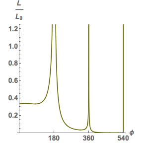 |
The change in apparent luminosity of individual stars, vs. φ, for a stationary observer at r = 3M. This is photons per unit area, not energy, so it doesn’t include the effect of the blue shift. There are spikes at multiples of 180°, where sin(φ) = 0; the first and widest spike is responsible for “Einstein rings”. Between the spikes are successively shallower troughs, for secondary images, tertiary images, etc. |
|
|
|