
A parabolic mirror will focus light rays arriving parallel to the mirror’s axis onto a single point: the focus of the mirror. But what happens more generally when light rays strike curved mirrors with other shapes?
If we confine ourselves to two dimensions, we can idealise the mirror as a curve in the plane, and plot out the reflected rays produced by light from a given source. In general, rather than passing through a single point, this family of reflected rays will have a curved “envelope” known as the catacaustic of the mirror curve.
I became interested in catacaustics thanks to a fascinating post on epicycloids on John Baez’s Azimuth blog, which pointed out that the catacaustic of a circle when the light source lies on the circle itself is a cardioid (an epicycloid with one cusp), and the catacaustic of a cardioid when the light source is placed at its cusp is a nephroid (an epicycloid with two cusps). Alas, this pattern doesn’t continue: the catacaustic of a nephroid is not another epicycloid, no matter where you place the light source.
In the disussion that followed, John Baez raised an interesting puzzle: if you have a mirror curve described by a polynomial of a certain degree, d, what is the maximum possible degree of the polynomial that describes its catacaustic? He later found a fairly high-powered algebraic geometry paper[1] that answered this question, and gave a precise formula for the degree of the catacaustic in every possible case. But while investigating the question myself, I had a lot of fun with some rather less daunting calculations. This page is a record of some of the fascinating results and methods I came across along the way ... and of course there are also plenty of nice pictures.

If you look carefully at the picture above, which shows a catacaustic of a second-degree curve (an ellipse), you can see that the degree of the catacaustic in this case must be at least six, because it’s possible to find a straight line that intersects the curve at six points.
The image on the right shows a catacaustic of the quartic curve:
x4 + y4 – x y = 1
This catacaustic has degree 36! After looking at lots of examples, my conjecture is that when the mirror curve has degree d, the maximum degree of the catacaustic is 3 d (d – 1). That conjecture is confirmed in [1], but so far I’ve been unable to construct a simple proof of it myself.
A parameterised curve in two dimensions is one for which we have an explicit description of the coordinates of every point on the curve in terms of two functions of a parameter, say t, which take its values in some interval of the real numbers. In general, the curve will be a set of the form:
{(x(t), y(t)) | t ∈ [a, b]}
We will assume that these coordinate functions x(t) and y(t) are continuous and twice differentiable; we say that such a curve is C 2. If there are a finite number of points where this fails it doesn’t really matter, as we can always break the curve into pieces and analyse the individual segments that are C 2. As a simple example, one parameterised description of a circle of radius R centred on the origin is:
{(R cos(t), R sin(t)) | t ∈ [0, 2π]}
The direction of the tangent to our parameterised curve at each point (x(t), y(t)) will be (x'(t), y'(t)). The parameterisation of any given curve is not unique, and it might be that at some points our particular parameterisation gives a vector of (x'(t), y'(t)) = (0, 0), even though the curve actually has a well-defined tangent. As with a failure to be C 2, as long as this only happens at a finite number of points it won’t really cause any problems. From the tangent, we can form a vector normal to the curve: (–y'(t), x'(t)).
We will assume that we have an idealised light source that occupies a point at the origin of our coordinate system. This will make the formulas that follow a bit simpler, and we can always deal with point sources at different locations by a change of coordinates.
How can we describe the reflection of a ray of light whose initial direction is along some vector v, in a mirror whose normal vector (a vector perpendicular to the surface) is n? Reflection simply reverses the component of v that is normal to the mirror, leaving the component parallel to the mirror unchanged. So we can find the reflected vector, say rn(v), by subtracting twice the normal component of v from v. If the normal vector was a unit vector u, the normal component of v would be (v · u) u, but more generally we can use a normal vector n of any length by setting u = n / |n|, so the normal component of v is (v · n) n / |n|2. The reflected vector is then:
rn(v) = v – 2 (v · n) n / |n|2
which satisfies the equation:
rn(v) · n = –v · n
With a light source at the origin, the initial direction of a ray from the source to each point on the curve is given by the coordinates of the point itself: v = (x(t), y(t)). Along with the normal at this point on the curve, n = (–y'(t), x'(t)), we have:
r(t) = (x(t), y(t)) – 2 [(x(t), y(t)) · (–y'(t), x'(t))] (–y'(t), x'(t)) / [x'(t)2 + y'(t)2]
= (x(t), y(t)) – 2 [x'(t) y(t) – y'(t) x(t)] (–y'(t), x'(t)) / [x'(t)2 + y'(t)2]
with:
r(t) · n = –(x(t), y(t)) · n
–rx(t) y'(t) + ry(t) x'(t) = x(t) y'(t) – y(t) x'(t)
Every point on this reflected ray will then take the form:
p(t, λ) = (x(t), y(t)) + λ r(t)
for some real number λ. If we were going to limit ourselves to the actual physical rays, we would restrict this to λ ≥ 0, but just as a convex mirror can have a virtual focus from which light rays appear to emerge even though no light is actually present there, we will include virtual catacaustics in our analysis: the envelope formed by those parts of the reflected ray where we continue it back behind the mirror. This makes the mathematics much simpler, and when we plot the whole curve it’s usually clear from inspection which part of the catacaustic is virtual.
Each point on the catacaustic itself will lie at the intersection of two “infinitesimally close” rays: that is, at the limit of the point of intersection of the lines given by p(t, λ) and p(t+δ, μ) as δ goes to zero. If we write r(t) = (rx(t), ry(t)), this amounts to solving the linear equations in λ and μ:
rx(t) λ – rx(t+δ) μ = x(t+δ) – x(t)
ry(t) λ – ry(t+δ) μ = y(t+δ) – y(t)
For sufficiently small δ this becomes:
rx(t) λ – [rx(t) + rx'(t) δ] μ = x'(t) δ
ry(t) λ – [ry(t) + ry'(t) δ] μ = y'(t) δ
This system is solved by:
λ = [(rx + rx' δ) y' – (ry + ry' δ) x'] / [ry rx' – rx ry']
μ = [rx y' – ry x'] / [ry rx' – rx ry']
= [y x' – x y'] / [ry rx' – rx ry']
where we’ve dropped the explicit mention of the parameter t to make the formulas a bit less crowded. When δ goes to zero, the point of intersection is given by:
C(t) = (x(t), y(t)) + [y x' – x y'] / [ry rx' – rx ry'] r(t)
This is the catacaustic of our mirror curve (x(t), y(t)), where r(t) = (rx(t), ry(t)) is the reflected ray derived above. If we switch the term y x' – x y' back to the original rx y' – ry x', this formula is independent of the details of our function r(t), and gives the envelope of any parameterised family of lines that pass through a parameterised curve (x(t), y(t)) and have direction r(t). Without using the definition of r(t), a straightforward calculation shows that C'(t) will always be parallel to r(t), i.e. the tangent to the envelope curve will always be parallel to the corresponding line in the family, as you’d expect.
A more general method to find the envelope of any family of lines or curves given implicitly by the condition G(t, X, Y) = 0, where t parameterises the family and we write (X, Y) for a point on the envelope curve, is to solve G(t, X, Y) = 0 simultaneously with ∂tG(t, X, Y) = 0. For our family of lines that pass through (x(t), y(t)) with direction r(t), that gives us:
G(t, X, Y) = [(X, Y) – (x(t), y(t))] · (–ry(t), rx(t)) = 0
∂tG(t, X, Y) = – (x'(t), y'(t)) · (–ry(t), rx(t)) + [(X, Y) – (x(t), y(t))] · (–ry'(t), rx'(t)) = 0
which is solved by:
(X, Y) = (x(t), y(t)) + [rx y' – ry x'] / [ry rx' – rx ry'] r(t)
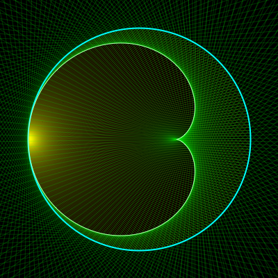
To make use of our formula for the catacaustic, let’s take the example of a circle of radius 1, with the light source on its rim. To allow the source to be at the origin as we’ve assumed, we will put the centre of the circle at (1, 0), so we have:
(x(t), y(t)) = (1 + cos(t), sin(t))
(x'(t), y'(t)) = (–sin(t), cos(t))
x'(t)2 + y'(t)2 = 1
r(t) = (x(t), y(t)) – 2 [x'(t) y(t) – y'(t) x(t)] (–y'(t), x'(t)) / [x'(t)2 + y'(t)2]
= (1 + cos(t), sin(t)) – 2 [–sin(t)2 – cos(t) – cos(t)2] (–cos(t), –sin(t))
= (1 + cos(t), sin(t)) – 2 [1 + cos(t)] (cos(t), sin(t))
= (1 – cos(t) – 2 cos(t)2, –sin(t) – 2 sin(t) cos(t))
= (–cos(t) – cos(2t), –sin(t) – sin(2t))
r'(t) = (sin(t) + 2 sin(2t), –cos(t) – 2 cos(2t))
y x' – x y' = –sin(t)2 – cos(t) – cos(t)2
= –1 – cos(t)
ry rx' – rx ry' = (–sin(t) – sin(2t)) (sin(t) + 2 sin(2t)) – (–cos(t) – cos(2t)) (–cos(t) – 2 cos(2t))
= –3 – 3 sin(2t) sin(t) – 3 cos(2t) cos(t)
= –3 – 3 cos(t)
C(t) = (x(t), y(t)) + [y x' – x y'] / [ry rx' – rx ry'] r(t)
= (1 + cos(t), sin(t)) + (1/3) (–cos(t) – cos(2t), –sin(t) – sin(2t))
= (1, 0) + (2/3) (cos(t), sin(t)) – (1/3) (cos(2t), sin(2t))
We can see that this is a cardioid, because apart from the offset of (1, 0) this is a point on a circle of radius 2/3 (and hence the location of the centre of one circle of radius 1/3, rolling around another of the same size) minus an offset from the centre of the rolling circle to a point on its rim, where the rolling circle rotates at twice the angular speed of its centre. This double-speed rotation means the tangential velocity of the point on the rim of the rolling circle is zero when it touches the fixed inner circle.
|
|
The top image on the left shows the catacaustic of a circle with the source on its rim. Yellow lines are drawn from the source to the mirror, and then the reflected rays are drawn in green (and extended in both directions from the point of reflection). The catacaustic, the envelope of the reflected rays, is shown in light green.
 |
 |
The top image on the right shows the catacaustic of a cardioid with the source located at its cusp, computed using the same methods as we used for the circle. In this case the catacaustic is a nephroid.
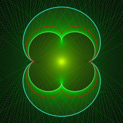
The bottom image on the left shows the catacaustic of a nephroid with the source at its centre. This looks a lot like a 4-cusped epicycloid, but an actual epicycloid is shown in red for comparison, making it clear that the shapes aren’t actually the same.
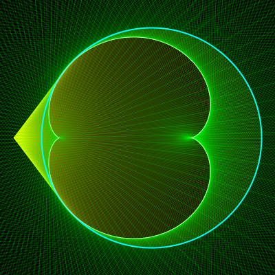
Finally, the bottom image on the right shows the catacaustic of a circle when the source is outside the circle. The portion of the curve which lies on the opposite side of the mirror to the source is a virtual catacaustic: it shows the curve along which the rays reflected from the mirror would appear to originate, even though no light would actually be present there.
Not all curves can be parameterised, but another useful way of describing curves is by means of an implicit equation:
P(x, y) = 0
for some function P of x and y. If P is a polynomial, we call the solution set:
{(x, y) | P(x, y) = 0}
a polynomial curve or an algebraic curve. The first example we gave of a parameterised curve, a circle of radius R, can also be described as a polynomial curve:
{(x, y) | x2 + y2 – R2 = 0}
The normal to a polynomial curve at some point (x, y) that lies on the curve is given by the gradient of the defining polynomial:
n = ∇P(x, y) = (∂x P(x, y), ∂y P(x, y))
Recalling our original formula for the reflection of a vector v in a mirror with normal n:
rn(v) = v – 2 (v · n) n / |n|2
we find the reflection of a ray from the origin to some point (x, y) on the curve to be:
r(x, y) = (x, y) – 2 ((x, y) · ∇P) ∇P / |∇P|2
with:
r(x, y) · ∇P = – (x, y) · ∇P
Now, we’re going to want to take the derivative of r(x, y) and also x and y themselves as we move along the curve. How can we do this? Despite not having an actual parameterisation of our polynomial curve, we can mimic a large part of the construction we used earlier for parameterised curves, simply by pretending that we have such a thing, and then making use of the following calculation:
P(x, y) = 0
∂t P(x(t), y(t)) = 0
∂x P(x, y) x'(t) + ∂y P(x, y) y'(t) = 0
y'(t) = –[∂x P / ∂y P] x'(t)
∂t r(x(t), y(t)) = ∂x r(x, y) x'(t) + ∂y r(x, y) y'(t)
= [∂x r – [∂x P / ∂y P] ∂y r] x'(t)
We can then adapt our formula for the catacaustic of a parameterised curve by using these expressions for derivatives with respect to the fictitious parameter t. Once everything is given in terms of x'(t), this cancels out of the formula and we’re left only with derivatives with respect to the actual coordinates.
C(x, y) = (x, y) + [y x' – x y'] / [ry rx' – rx ry'] r(x, y)
= (x, y) + [y + x [∂x P / ∂y P]] / [ry [∂x rx – [∂x P / ∂y P] ∂y rx] – rx [∂x ry – [∂x P / ∂y P] ∂y ry]] r(x, y)
This gives us finally:
C(x, y) = (x, y) + ((x, y) · ∇P) / [ry [∂x rx ∂y P – ∂y rx ∂x P] – rx [∂x ry ∂y P – ∂y ry ∂x P]] r(x, y)
This is the point on the catacaustic associated with the point (x, y) on the mirror.
This might not seem very useful, since in the absence of a parameterisation we have no supply of actual points on the mirror! But let’s work through a simple example and see where it gets us.
We’ll look once again at the case of a unit circle with its centre at (1, 0). We have:
P(x, y) = (x – 1)2 + y2 – 1
∇P = 2 (x – 1, y)
|∇P|2 = 4 ((x – 1)2 + y2)
(x, y) · ∇P = 2 (x2 – x + y2)
r(x, y) = (x, y) – 2 ((x, y) · ∇P) ∇P / |∇P|2
= (x, y) – 2 [(x2 – x + y2) / ((x – 1)2 + y2)] (x – 1, y)
∂x r = (–(x – 1)4 – 2 (x2 – 1) y2 – y4, 2 y (x – y – 1)(x + y – 1)) / [(x – 1)2 + y2]2
∂y r = (4 (x – 1)2 y, –(x – 1)3 (x + 1) – 2 (x – 2) (x – 1) y2 – y4) / [(x – 1)2 + y2]2
C(x, y) = (x, y) + ((x, y) · ∇P) / [ry [∂x rx ∂y P – ∂y rx ∂x P] – rx [∂x ry ∂y P – ∂y ry ∂x P]] r(x, y)
= 2 ((x – 1)2 x2 + (2 x – 1) x y2 + y4, y3) / [((x – 1)2 + y2) (x2 + x + y2)]
What can we do with this result? Our aim is to find a polynomial Q such that Q(X, Y) = 0 given (X, Y) = C(x, y) and P(x, y) = 0. In other words, we want to eliminate the variables x and y from the system of simultaneous equations in x, y, X and Y:
(x – 1)2 + y2 – 1 = 0
X [((x – 1)2 + y2) (x2 + x + y2)] – 2 [(x – 1)2 x2 + (2 x – 1) x y2 + y4] = 0
Y [((x – 1)2 + y2) (x2 + x + y2)] – 2 y3 = 0
It’s not too hard to tackle this particular system: we can easily solve the first equation for y2 and substitute the result into the other equations. This gives us a new version of the third equation that we can then solve for y itself, so that’s one variable eliminated. A similar strategy with x2 and x lets us finish the job, and the result is:
x = (–9/4) (X 2 – 2 X + Y 2)
y = (3/2) Y / (2 – x)
x (–64 X + 144 X 2 – 108 X 3 + 27 X 4 + 36 Y 2 – 108 X Y 2 + 54 X 2 Y 2 + 27 Y 4) = 0
Although we’ve found an expression for x in terms of X and Y, it’s easier to understand what’s going on with the first factor in the last line here if we leave it as it is. Since x = 0 only solves the full set of equations for a single point on the mirror curve, x = y = 0, we can discard that factor, and the remaining polynomial in X and Y alone describes the catacaustic.
More generally, we can eliminate variables from a system of polynomial equations like this by constructing a suitable Gröbner basis[2] that generates the same set of polynomials as generated by the three listed above.
This requires some explanation! In this context, a basis is a (usually finite) set of polynomials, and we say that the polynomials generated by a basis are those that can be formed by taking polynomial-linear combinations of elements of the basis, i.e. by multiplying elements of the basis by any polynomials we like in the same variables, and adding the results together.
A Gröbner basis is one that satisfies the property that the leading term of any polynomial in the set generated by the basis has equal or higher powers of all variables compared to the leading term of at least one element of the basis. For example, if the set generated by the basis contains a polynomial with the leading term 72 x y X 2 Y 3, then at least one element of the basis will have a leading term with the powers of all variables less than or equal to those in x y X 2 Y 3.
What exactly is the “leading term” of a polynomial in several variables? When there’s only one variable we usually say that the leading term is simply the one with the highest power of that variable, but how should we compare X 4 Y and Y 4 X? The answer is that we need to choose some ordering, and the scheme we choose will be arbitrary, but we can nevertheless make a choice that’s useful for our particular purpose. If we use the ordering scheme known as lexicographic order, we first choose an order for the individual variables — say, X < Y < x < y – and then terms are sorted so that the mere presence of a higher-ranked variable counts for more than the highest exponent of any lower-ranked variable. For example, with our ordering, X 100 < x. If we construct a Gröbner basis from our three polynomials with this ordering scheme, then it will end up including a polynomial with a factor that’s free of the higher-ranked variables x and y. (For more detail, including a description of the algorithm for constructing a Gröbner basis, see the Scholarpedia article.)
If we use a computer algebra package to generate the Gröbner basis in this way for the polynomials in our example, it will contain the element:
x (–64 X + 144 X 2 – 108 X 3 + 27 X 4 + 36 Y 2 – 108 X Y 2 + 54 X 2 Y 2 + 27 Y 4)
As we argued previously, it’s appropriate to discard the factor of x and set Q(X, Y) equal to the second factor. As a check, if we substitute the expressions we found for X and Y in terms of x and y into Q(X, Y), the result turns out to contain a factor of P(x, y) = (x – 1)2 + y2 – 1, and so P(x, y) = 0 will imply Q(X, Y) = 0. We can also check this result by substituting in the answer we found for the parameterised form of the same catacaustic:
Q(1 + (2/3) cos(t) – (1/3) cos(2t), (2/3) sin(t) – (1/3) sin(2t))
This turns out to be zero for all t.
The approach we’ve shown here provides a reasonably practical way to find the catacaustics in particular cases, especially if you have access to suitable software for creating Gröbner bases. But the algorithm used to do that is complicated, and the method doesn’t really give us much insight into the geometry of these curves. So in the next few sections, we’ll take a detour and consider a more geometrical approach.

If two curves in the plane intersect but don’t share a tangent, they are described as making 0th-order or 1-point contact.
If two curves intersect and do share a tangent, they are said to make (at least) 1st-order or 2-point contact.
If two curves intersect and share an osculating circle, they make (at least) 2nd-order or 3-point contact. An osculating circle to a curve is a circle whose radius matches the radius of curvature of the curve, and whose centre is positioned so that the curve and the circle share a tangent where they intersect.
Why say that curves sharing a tangent make “2-point contact” if they only intersect at one point? If you take any two points on a curve, you can always draw a straight line that passes through both of them. As the two points come closer together, in the limiting case where they coincide that line becomes the tangent there. So two curves sharing a tangent line are sharing “two” (infinitesimally close) points.
It might sound as if the double nature of the intersection disappears when the two points end up as one, but it remains in the following sense. If the curves are defined implicitly, say by polynomials P(x, y) = 0 and Q(x, y) = 0, if we evaluate these functions along the shared tangent by setting y = a x + b with suitable values for a and b, then the polynomials in x we get this way, P(x, a x + b) and Q(x, a x + b), will have a double root in common at the point of intersection, i.e. they will share a factor of (x – x0)2 where (x0, a x0 + b) is the point of intersection. More generally, even if P and Q are not polynomials, both functions evaluated along the shared tangent line will be zero to 1st order at x0: that is, their derivatives at x0 will be zero, as well as the functions themselves, so the first term in their Taylor series there will be a multiple of (x – x0)2.
Similarly, if you take any three points on a curve, then (so long as they’re not collinear), you can always find a circle that passes through all three of them. In the limiting case where the three points coincide, this circle becomes an osculating circle for the curve. For two curves with three-point contact defined by P(x, y) = 0 and Q(x, y) = 0, we can evaluate P and Q along the curves’ shared osculating circle by treating the circle as a parameterised curve, say with an angular parameter θ. The functions of θ we obtain this way will be zero to 2nd order at the point of intersection, with both the first and second derivatives zero there, and so the first term in their Taylor series will be a multiple of (θ – θ0)3. In that sense, curves with three-point contact have a kind of triple intersection.
A circle in the plane is completely determined by three parameters: the two coordinates of its centre, and its radius. This is why it’s possible to find a circle that passes through three arbitrary points, or to find a circle that makes 3-point contact with a curve. But if we consider some other three-parameter family of curves, we can single out one of them in the same way: by requiring that the curve makes 3-point contact with another curve at some particular point. The family of curves that will be of interest to us are conic sections, or conics for short: these include circles, parabolas and pairs of lines as special cases, but generically are either ellipses or hyperbolas. Every conic section can be defined implicitly by a quadratic equation of the form:
A x2 + B x y + C y2 + D x + E y + F = 0
There are six parameters in this equation, but because we can multiply the equation through by any non-zero number without changing the curve it defines, there are really only five parameters that fix the geometry of the curve.

The three-parameter family that we’re interested in will consist of all conics that have one of their foci at a particular point, which for the sake of simplicity we will place at the coordinate origin (0, 0). The remaining three parameters are then the two coordinates of the other focus, say (X, Y), and a parameter that sets the size of the curve, which we will call γ.
The image on the left shows a set of conics with foci at (0, 0) and (2, 3), and a range of values for the third parameter.
Any member of the full three-parameter family can be described by a quadratic of the form:
8 x X y Y + 4 x X γ + 4 y Y γ + γ2 – 4 y2 (X 2 + γ) – 4 x2 (Y 2 + γ) = 0
This conic has one focus at (0, 0) and one at (X, Y). Its major and minor semi-axes a and b are:
a = ½ √(X 2 + Y 2 + γ)
b = ½ √|γ|
The distance between the foci is obviously √(X 2 + Y 2), and in the geometry of conics half this distance is often given the name c:
c = ½ √(X 2 + Y 2)
A conic is an ellipse when the major axis is greater than the distance between the foci, i.e. when a > c, which in terms of our parameters will be true when γ > 0.
When a < c the conic becomes a hyperbola, which in our terms will happen when γ < 0.
In the case a = c or γ = 0, our conic degenerates into:
(X y – Y x)2 = 0
This is a single line running through both foci (the dashed grey line in the image). In the case a = 0 or γ = –X 2 – Y 2, our conic degenerates into:
(X 2 + Y 2 – 2 X x – 2 Y y)2 = 0
This is a single line orthogonal to, and bisecting, the line segment between the foci (the dashed black line in the image). It’s worth noting that although, geometrically, these two degenerate cases appear as single lines, the fact that the expression we get is squared means these lines are in a sense doubled, in the same way that an intersection between curves making 2-point contact is doubled.
 |
 |
Now, conics have a very interesting property as mirror curves. If we place a light source at one focus of an ellipse (top image on the left), every single ray that leaves the source will be reflected so that it passes through the other focus.
If we place a light source at one focus of a hyperbola (bottom image on the left), every ray that leaves the source will be reflected so that it appears to emerge from the other focus – it will be a virtual focus for the rays.
This is why our family of conics with one focus fixed can tell us something about the catacaustic of a curve:
| If a conic with one focus at the light source makes 3-point contact with a curve, then the other focus of the conic will lie on the catacaustic for the curve. |
Why is this true? If two curves make 2-point contact that means they share a tangent, and any single light ray that is reflected from one curve at the point of intersection will be reflected in exactly the same way from the second curve, with the shared tangent acting like the mirror at that point.
But if two curves make 3-point contact, we can go one step further: in the limit of two rays that come ever closer to the point of intersection of the curves, both rays will be reflected identically from the two curves, and they will end up meeting each other at the same point regardless of the curve we use to reflect them. In the case that one of the two curves is a conic with one focus at the light source, we know that all the rays it reflects will end up meeting at the other focus. So the rays reflected from the second curve must also meet there, which means that the other focus of the conic will coincide with a point on the second curve’s catacaustic.
 |
The image on the right shows a succession of ellipses with one focus at the source making 3-point contact with a circular mirror curve. The second focus of each ellipse always lies on the catacaustic of the mirror curve.
(What happens when the catacaustic has a cusp – when the curve seems to linger at one point, coming a bit closer than usual to bringing the rays to a single focus? At these points, the osculating conic makes 4-point contact: there is agreement between the conic and the mirror curve to third order.)
We now have another way of thinking about the polynomial equation Q(X, Y) = 0 that is satisfied by all points (X, Y) on the catacaustic. If we chose any old (X, Y) for the second focus of our conic, then as we varied the parameter γ we would find that there was generally at least one value that made the conic tangent to the mirror curve. It’s only for those special values of (X, Y) satisfying Q(X, Y) = 0 that varying γ lets us find a conic making 3-point contact.
But we still need a method to determine exactly what the condition Q(X, Y) = 0 should be in order that the conic has this property – and this is where resultants come into the story.
Suppose we’re given two polynomials in the same variable, say p(x) and q(x). Is there are any way to know whether p and q have a root in common, without actually solving both polynomials and listing all their roots? Surprisingly enough, there is! It’s possible to compute a quantity called the resultant[4][5] of p and q that can be found from their coefficients using only addition, subtraction and multiplication, and which is zero if and only if they have at least one root in common. The most straightforward way to compute the resultant is as the determinant of a matrix known as the Sylvester matrix.
Suppose p has degree m and q has degree n, with coefficients pi, qi:
p(x) = pm xm + pm–1 xm–1 + ... + p2 x2 + p1 x + p0
q(x) = qn xn + qn–1 xn–1 + ... + q2 x2 + q1 x + q0
Then the Sylvester matrix is a square matrix of size (m + n) × (m + n), with n rows consisting of the coefficients of p in descending order shifted forward along the row by varying amounts from 0 to n–1 until the last entry in the row is p0, followed by m rows consisting of the coefficients of q in descending order shifted forward along the row by varying amounts from 0 to m–1, until the last entry in the row is q0:
| Syl(p, q, x) | = |
|
We write Syl(p, q, x) and specify the variable x to make it clear that these coefficients refer to powers of x. If p and q are polynomials in more than one variable, we can still construct a Sylvester matrix for them in any one of their variables, but in that case each of these matrix entries will include the other variables as part of the coefficient.
How can the Sylvester matrix tell us when p and q have a common root? For some number α, consider the (m+n)-dimensional vector of descending powers of α, starting from αm+n–1:
v(α) = (αm+n–1, αm+n–2, ..., α2, α, 1)
If we multiply this by Syl(p, q, x), we get:
|
|
= |
|
If p(α) = q(α) = 0, then this product will be the zero vector. But v(α) is never the zero vector, because there’s always at least the entry of 1 at the end. The only way a matrix can have a non-trivial null space (that is, the only way it can produce zero from a non-zero vector) is if its determinant is zero. So we define the Sylvester resultant of p and q to be:
Res(p, q, x) = Det(Syl(p, q, x))
We’ve shown that if p and q have a root in common, the resultant is zero. And though we won’t prove it, the converse is also true: if the resultant is zero, p and q must have (at least) one root in common.
This assumes that we’ve correctly identified the degrees of the polynomials. If the leading coefficients of both polynomials are actually zero, pm = qn = 0 (which might sound like a silly mistake, but if the coefficients are themselves defined in terms of other parameters, the leading coefficients might well be zero for some values of those parameters), then the first column of the Sylvester matrix will be zero and so its determinant will be zero, regardless of whether the polynomials have a common root.
If we truncate the Sylvester matrix by discarding the last two columns, and the last row of each block derived from each of the two polynomials, we end up with a matrix of size (m + n – 2) × (m + n – 2) that we will call Syl1(p, q, x):
| Syl1(p, q, x) | = |
|
We define the subresultant as the determinant of the truncated matrix:
SubRes(p, q, x) = Det(Syl1(p, q, x))
The resultant and the subresultant of a pair of polynomials are both zero if and only if the polynomials have (at least) two roots in common, counted by multiplicity. That is to say, both polynomials are divisible by a factor of (x–α)(x–β), but it’s possible that β=α and the common factor is (x–α)2.
Finally, one very useful specialisation of the resultant is the discriminant, which is defined as the resultant of a polynomial with its own derivative, divided by the polynomial’s leading coefficient:
Disc(p, x) = Res(p, ∂x p, x) / pm
If a polynomial has a double root, it will share that root with its derivative:
p(x) = (x – α)2 f(x)
p'(x) = 2 (x – α) f(x) + (x – α)2 f '(x)
= (x – α) [2 f(x) + (x – α) f '(x)]
A shared root means the resultant is zero, so the discriminant of a polynomial with a double root is zero. We divide out the leading coefficient pm because the leading coefficient of the derivative will be m pm, making it a common factor in the determinant.
We’re now in a position to use resultants and discriminants to help us construct the implicit equation for the catacaustic of a polynomial curve.
We’ll refer to a member of our three-parameter family of conics as F(x, y), with:
F(x, y) = 8 x X y Y + 4 x X γ + 4 y Y γ + γ2 – 4 y2 (X 2 + γ) – 4 x2 (Y 2 + γ)
while the mirror curve will be described by P(x, y) = 0. Also, we’ll define:
Resy(x) = Res(P, F, y)
Resx(y) = Res(P, F, x)
and similarly for subresultants SubResy(x) and SubResx(y), where in each case the coordinate with respect to which we take the resultant or subresultant is eliminated, leaving a function of the other coordinate. Of course both these resultants also still depend (via F) on our three parameters, X, Y and γ.
Suppose the two curves P(x, y) = 0 and F(x, y) = 0 intersect at some point (x0, y0). Then their common root will show up as a zero in the resultant with respect to either variable, x or y. The resultant Resy(x), which treats the two polynomials as functions of y (with coefficients that are functions of x) will equal zero when x=x0, since the two polynomials in y along the vertical line x=x0, namely P(x0, y) and F(x0, y), will share a common root at y=y0.
Similarly, Resx(y), which treats the two polynomials as functions of x (with coefficients that are functions of y) will equal zero when y=y0, since the two polynomials in x along the horizontal line y=y0, namely P(x, y0) and F(x, y0), will share a common root at x=x0.
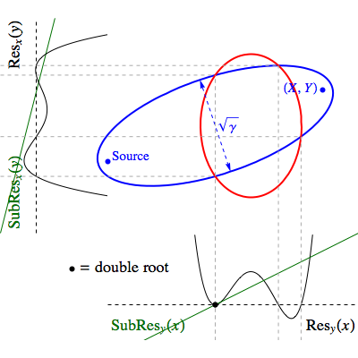
In the image on the left, the red ellipse is the mirror curve, while the blue ellipse belongs to our three-parameter family of conics with one focus at the origin. Every point of intersection between the curves shows up as a zero in both resultants.
We’ve chosen an example where two of the intersections lie on a vertical line, so there is a double root there for the corresponding resultant. What’s more, at that root the subresultant is also zero, because along that vertical line P(x0, y) and F(x0, y) share two roots.

Now, suppose the curves P(x, y) = 0 and F(x, y) = 0 make 2-point contact at (x0, y0), so as well as intersecting they share a tangent there, as in the image on the right. Generally, the functions P(x0, y) and P(x, y0) won’t have double roots; it’s only when you evaluate a function P(x, y) along its tangent line that its derivative vanishes where the tangent meets the curve P(x, y) = 0. However, the resultant functions, which have zeroes at every point of intersection between the curves, will have double roots, with Resy(x) having a double root at x=x0 and Resx(y) having a double root at y=y0.
The discriminants of these resultants will tell us whether or not they have double roots, and either one will do. However, as we’ve seen, if the two curves happen to have two separate intersections that lie on the same vertical or horizontal line, then that will also produce a double root in one of the resultants.
So to find a polynomial in X, Y and γ that will be zero only when there’s 2-point contact, we take Disc(Resy(x), x), which is zero whenever Resy(x) possesses double roots, and divide it by Res(Resy(x), SubResy(x), x), which is zero if the resultant and subresultant have any roots in common. This removes the factors that are due to vertically aligned pairs of separate intersections.
There is one more catch to consider: with certain values for the parameters (namely γ=0 or γ = –X 2 – Y 2), our conics degenerate into double lines, and every intersection they have with another curve is a double intersection. So there will always be factors of γ and (γ + X 2 + Y 2) in Disc(Resy(x), x), and we need to divide them out as well to find the true condition for the conic to be tangent to the curve. A polynomial curve of degree d will intersect a generic line at d points (including complex-valued points), so we need to divide out that many factors.
Accordingly, we’ll define:
Tangency(X, Y, γ) = Disc(Resy(x), x) / [Res(Resy(x), SubResy(x), x) (γ + X 2 + Y 2)d γd]
where d is the degree of the mirror curve P.
If we fix the values of X and Y then Tangency(X, Y, γ) becomes a polynomial in γ, and in general it will have a number of single roots, each of which specifies a conic that is simply tangent to the mirror curve.
If we go on to compute Disc(Tangency(X, Y, γ), γ), this discriminant will be zero when the values of X and Y allow for a double root in γ, implying a higher order of contact.
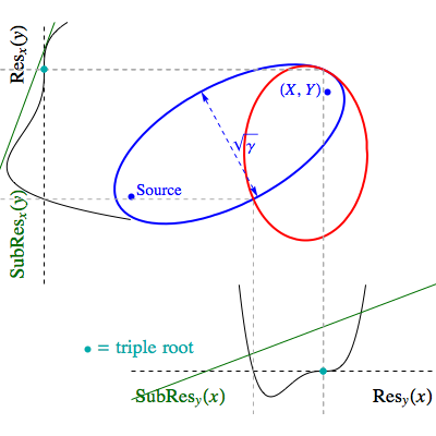
Sometimes a double root in γ will entail genuine 3-point contact between the conic and the mirror curve, as in the image on the left. Here, the values of X and Y have been chosen so that Disc(Tangency(X, Y, γ), γ) = 0, ensuring that there is a double root in γ, and the blue ellipse is drawn for γ lying exactly on that double root. Because the curves make 3-point contact (which shows up as a triple root in the resultants along the coordinate axes), the chosen (X, Y) definitely belongs to the catacaustic.

However, sometimes there will be a double root in γ simply because the conic is tangent to the mirror curve at two locations simultaneously, as in the image on the right. (X, Y) here does not belong to the catacaustic, despite Disc(Tangency(X, Y, γ), γ) being zero.
It might seem surprising at first that we can achieve two 2-point contacts with a three-parameter family of curves – shouldn’t we need four parameters? But the fourth parameter is provided by the freedom to put the second 2-point contact anywhere at all on the mirror curve: for every point where we require the conic to be a tangent, not only can we vary X, Y and γ, we can vary the location of the other point of tangency.
Alas, I’m unable to obtain an explicit formula for the factors that need to be removed from Disc(Tangency(X, Y, γ), γ) in order to isolate the catacaustic itself. According to the paper Explicit Factors of Some Iterated Resultants and Discriminants[3], a discriminant of a discriminant should factor into three parts:
Discy(Discz(f)) = A B3 C2
Sample calculations show that Disc(Tangency(X, Y, γ), γ) does indeed factor in exactly that form, with the polynomial that turns out to be the catacaustic Q(X, Y) appearing with an exponent of 3, and another polynomial that gives double tangents appearing with an exponent of 2. The third factor seems to be a kind of artifact of the parameterisation of the conics. So this method ultimately does yield the catacaustic, and it’s not hard to see which term it is.

The image on the left shows curves of Tangency(X, Y, γ) = 0 for various values of γ, and it’s clear that the catacaustic (the blue curve in the middle) consists of all points where the Tangency curves have cusps. These curves also contain self-intersections — which are the points where the conic has two separate 2-point contacts with the mirror curve. The two cases can be distinguished by the determinant of the Hessian matrix of second partial derivatives, which is zero for the cusps, but it’s not clear how to use this to isolate the catacaustic in a straightforward way. Points on the catacaustic will be, for some value of γ, points where the Tangency function, its derivatives with respect to both X and Y, and the determinant of its Hessian are all zero, and the resultants with respect to γ of any two of these functions will include the catacaustic as a factor, but as with Disc(Tangency(X, Y, γ), γ) there are always extraneous factors as well.
In theory, there must be a polynomial whose zero set consists only of those (X, Y) values such that Resy(x) has a triple root for some x and γ ... and of course there is, because that’s precisely what the catacaustic is! We can describe this in an abstract sense as:
Q(X, Y) = Resx, γ(Resy(x), Resy'(x), Resy''(x))
That is, it’s a polynomial in X and Y that when zero guarantees that all three of these functions share a root for some x and γ. However, I’m not aware of any practical means of computing this directly; I’ve tried using the Macaulay resultant[5] but this also gives extraneous factors, and sometimes the determinants are uniformly zero. Maybe when I get around to reading the magnum opus[4] by Gelfand, Kapranov and Zelevinsky that everyone cites on this subject, I’ll understand it well enough to make some more progress.
For practical purposes the Gröbner basis method is probably the most efficient. But this detour into kissing conics was more fun, and has revealed much more about the geometry of catacaustics.
Below is a worked example of the resultant method, using the red ellipse from the figures above as the mirror curve.
P(x, y) = 29 – 32 x + 8 x2 – 4 y + 4 y2
F(x, y) = 8 x X y Y + 4 x X γ + 4 y Y γ + γ2 – 4 y2 (X 2 + γ) – 4 x2 (Y 2 + γ)
The Sylvester matrix Syl(P, F, y) is:
4 –4 29 – 32 x + 8 x2 0 0 4 –4 29 – 32 x + 8 x2 –4 (X 2 + γ) 8 x X Y + 4 Y γ 4 x X γ + γ2 – 4 x2 (Y 2 + γ) 0 0 –4 (X 2 + γ) 8 x X Y + 4 Y γ 4 x X γ + γ2 – 4 x2 (Y 2 + γ)
Resy(x) = Det(Syl(P, F, y)) =
16 (841 X 4 – 1856 x X 4 + 1488 x2 X 4 – 512 x3 X 4 + 64 x4 X 4 – 232 x X 3 Y + 256 x2 X 3 Y – 64 x3 X 3 Y + 248 x2 X 2 Y 2 – 256 x3 X 2 Y 2 + 64 x4 X 2 Y 2 – 32 x3 X Y 3 + 16 x4 Y 4 + 1682 X 2 γ – 3712 x X 2 γ + 2760 x2 X 2 γ – 768 x3 X 2 γ + 64 x4 X 2 γ + 216 x X 3 γ – 256 x2 X 3 γ + 64 x3 X 3 γ – 232 x X Y γ + 256 x2 X Y γ – 96 x3 X Y γ – 116 X 2 Y γ + 128 x X 2 Y γ – 216 x2 Y 2 γ + 256 x3 Y 2 γ – 32 x4 Y 2 γ + 464 x X Y 2 γ – 512 x2 X Y 2 γ + 96 x3 X Y 2 γ – 16 x2 Y 3 γ + 841 γ2 – 1856 x γ2 + 1272 x2 γ2 – 256 x3 γ2 + 16 x4 γ2 + 216 x X γ2 – 256 x2 X γ2 + 32 x3 X γ2 + 54 X 2 γ2 – 64 x X 2 γ2 + 32 x2 X 2 γ2 – 116 Y γ2 + 128 x Y γ2 – 48 x2 Y γ2 + 24 x X Y γ2 + 116 Y 2 γ2 – 128 x Y 2 γ2 + 24 x2 Y 2 γ2 + 54 γ3 – 64 x γ3 + 8 x2 γ3 + 8 x X γ3 + 4 Y γ3 + γ4)
The truncated Sylvester matrix Syl1(P, F, y) is:
4 –4 –4 (X 2 + γ) 8 x X Y + 4 Y γ
SubResy(x) = Det(Syl1(P, F, y)) = –16 (X 2 – 2 x X Y + γ – Y γ)
Disc(Resy(x), x) =
1125899906842624 (X 2 + Y 2 + γ)2 γ2
(2 X 6 – 16 X 5 Y + 28 X 4 Y 2 + 5 X 4 γ – 32 X 3 Y γ – 2 X 4 Y γ + 27 X 2 Y 2 γ + 16 X 3 Y 2 γ + 2 X 2 Y 3 γ + 4 X 2 γ2 – 16 X Y γ2 – 4 X 2 Y γ2 – Y 2 γ2 + 16 X Y 2 γ2 + X 2 Y 2 γ2 + 2 Y 3 γ2 – Y 4 γ2 + γ3 – 2 Y γ3 + Y 2 γ3)2
(7569 X 4 – 8352 X 5 + 2088 X 6 + 40368 X 3 Y – 45588 X 4 Y + 11136 X 5 Y – 16820 X 2 Y 2 + 12992 X 3 Y 2 – 3596 X 4 Y 2 – 188384 X Y 3 + 210192 X 2 Y 3 – 46400 X 3 Y 3 + 164836 Y 4 – 155904 X Y 4 + 43152 X 2 Y 4 – 22736 Y 5 – 25984 X Y 5 + 22736 Y 6 + 139606 X 2 γ – 221328 X 3 γ + 111282 X 4 γ – 17888 X 5 γ – 148016 X Y γ + 248356 X 2 Y γ – 152608 X 3 Y γ + 31340 X 4 Y γ + 454140 Y 2 γ – 749824 X Y 2 γ + 431384 X 2 Y 2 γ – 85632 X 3 Y 2 γ – 123192 Y 3 γ + 100928 X Y 3 γ – 8560 X 2 Y 3 γ + 57384 Y 4 γ – 31616 X Y 4 γ – 9360 Y 5 γ + 296873 γ2 – 583248 X γ2 + 390274 X 2 γ2 – 103904 X 3 γ2 + 8785 X 4 γ2 – 91408 Y γ2 + 144592 X Y γ2 – 80328 X 2 Y γ2 + 16048 X 3 Y γ2 – 33100 Y 2 γ2 + 44288 X Y 2 γ2 – 16628 X 2 Y 2 γ2 + 1776 Y 3 γ2 + 4896 X Y 3 γ2 – 5820 Y 4 γ2 – 66492 γ3 + 90320 X γ3 – 39302 X 2 γ3 + 5424 X 3 γ3 + 11808 Y γ3 – 10000 X Y γ3 + 2468 X 2 Y γ3 – 2556 Y 2 γ3 + 128 X Y 2 γ3 + 648 Y 3 γ3 + 4222 γ4 – 3760 X γ4 + 814 X 2 γ4 – 272 Y γ4 + 112 X Y γ4 + 76 Y 2 γ4 – 108 γ5 + 48 X γ5 + γ6)
Res(Resy(x), SubResy(x), x) =
16777216 (2 X 6 – 16 X 5 Y + 28 X 4 Y 2 + 5 X 4 γ – 32 X 3 Y γ – 2 X 4 Y γ + 27 X 2 Y 2 γ + 16 X 3 Y 2 γ + 2 X 2 Y 3 γ + 4 X 2 γ2 – 16 X Y γ2 – 4 X 2 Y γ2 – Y 2 γ2 + 16 X Y 2 γ2 + X 2 Y 2 γ2 + 2 Y 3 γ2 – Y 4 γ2 + γ3 – 2 Y γ3 + Y 2 γ3)2
Tangency(X, Y, γ) = Disc(Resy(x), x) / [Res(Resy(x), SubResy(x), x) (X 2 + Y 2 + γ)2 γ2] =
67108864 (7569 X 4 – 8352 X 5 + 2088 X 6 + 40368 X 3 Y – 45588 X 4 Y + 11136 X 5 Y – 16820 X 2 Y 2 + 12992 X 3 Y 2 – 3596 X 4 Y 2 – 188384 X Y 3 + 210192 X 2 Y 3 – 46400 X 3 Y 3 + 164836 Y 4 – 155904 X Y 4 + 43152 X 2 Y 4 – 22736 Y 5 – 25984 X Y 5 + 22736 Y 6 + 139606 X 2 γ – 221328 X 3 γ + 111282 X 4 γ – 17888 X 5 γ – 148016 X Y γ + 248356 X 2 Y γ – 152608 X 3 Y γ + 31340 X 4 Y γ + 454140 Y 2 γ – 749824 X Y 2 γ + 431384 X 2 Y 2 γ – 85632 X 3 Y 2 γ – 123192 Y 3 γ + 100928 X Y 3 γ – 8560 X 2 Y 3 γ + 57384 Y 4 γ – 31616 X Y 4 γ – 9360 Y 5 γ + 296873 γ2 – 583248 X γ2 + 390274 X 2 γ2 – 103904 X 3 γ2 + 8785 X 4 γ2 – 91408 Y γ2 + 144592 X Y γ2 – 80328 X 2 Y γ2 + 16048 X 3 Y γ2 – 33100 Y 2 γ2 + 44288 X Y 2 γ2 – 16628 X 2 Y 2 γ2 + 1776 Y 3 γ2 + 4896 X Y 3 γ2 – 5820 Y 4 γ2 – 66492 γ3 + 90320 X γ3 – 39302 X 2 γ3 + 5424 X 3 γ3 + 11808 Y γ3 – 10000 X Y γ3 + 2468 X 2 Y γ3 – 2556 Y 2 γ3 + 128 X Y 2 γ3 + 648 Y 3 γ3 + 4222 γ4 – 3760 X γ4 + 814 X 2 γ4 – 272 Y γ4 + 112 X Y γ4 + 76 Y 2 γ4 – 108 γ5 + 48 X γ5 + γ6)
Disc(Tangency(X, Y, γ), γ) =
21430066217365073813580314159646942938899050443293914093809055644932287896169956245504
(16 X 2 – 8 X 3 + X 4 – 68 X Y + 17 X 2 Y – 16 Y 2 + 68 X Y 2 – 17 X 2 Y 2 + 32 Y 3 – 16 Y 4)2
(142041536 – 406021344 X + 495981084 X 2 – 333022016 X 3 + 129901296 X 4 – 27896856 X 5 + 2568437 X 6 – 188599296 Y + 388070112 X Y – 308560440 X 2 Y + 115942560 X 3 Y – 19272516 X 4 Y + 892824 X 5 Y + 190303104 Y 2 – 334833504 X Y 2 + 227128284 X 2 Y 2 – 72614976 X 3 Y 2 + 9357114 X 4 Y 2 – 96352576 Y 3 + 102821280 X Y 3 – 30815184 X 2 Y 3 + 1550432 X 3 Y 3 + 52485024 Y 4 – 42319776 X Y 4 + 10533756 X 2 Y 4 – 12527472 Y 5 + 683232 X Y 5 + 3774680 Y 6)3
(353 – 608 X + 408 X 2 – 128 X 3 + 16 X 4 – 120 Y + 128 X Y – 32 X 2 Y + 136 Y 2 – 128 X Y 2 + 32 X 2 Y 2 – 32 Y 3 + 16 Y 4)
Q(X, Y) = factor that appears cubed in Disc(Tangency(X, Y, γ), γ) =
142041536 – 406021344 X + 495981084 X 2 – 333022016 X 3 + 129901296 X 4 – 27896856 X 5 + 2568437 X 6 – 188599296 Y + 388070112 X Y – 308560440 X 2 Y + 115942560 X 3 Y – 19272516 X 4 Y + 892824 X 5 Y + 190303104 Y 2 – 334833504 X Y 2 + 227128284 X 2 Y 2 – 72614976 X 3 Y 2 + 9357114 X 4 Y 2 – 96352576 Y 3 + 102821280 X Y 3 – 30815184 X 2 Y 3 + 1550432 X 3 Y 3 + 52485024 Y 4 – 42319776 X Y 4 + 10533756 X 2 Y 4 – 12527472 Y 5 + 683232 X Y 5 + 3774680 Y 6
The final result here for the catacaustic is a curve of degree six. This is plotted as the curve in the middle of the last diagram before the calculations.
[1] On the Degree of Caustics of Reflection, Alfrederic Josse and Françoise Pène, online at arXiv preprint server.
[2] Gröbner basis, Bruno Buchberger and Manuel Kauers (2010), Scholarpedia, 5(10):7763, online at Scholarpedia.
[3] Explicit Factors of Some Iterated Resultants and Discriminants, Laurent Busé and Bernard Mourrain, online at arXiv preprint server.
[4] Discriminants, resultants, and multi-dimensional determinants, I. M. Gelfand, M. M. Kapranov, and A. V. Zelevinsky, Birkhäuser, 1994.
[5] An Introduction to the Theory of Resultants, Peter F. Stiller, Institute for Scientific Computation, Texas A & M University, PDF online.