This applet plots the roots (outside a certain annulus in the complex plane) of all the Littlewood polynomials of a given degree.
In 2006, Dan Christensen and Sam Derbyshire discovered the beautiful fractal patterns that can be found by plotting roots of polynomials like this. For more details (and some stunning pictures) see John Baez’s blog post. For some screen shots from this applet, see below. I’ve also made some related videos.
The Littlewood polynomials are polynomials of one variable with all their coefficients equal to ±1, e.g. L(z)=1+z–z2–z3+z4. Since the overall sign of the polynomial has no effect on the set of roots, it will be convenient to choose a specific subset of the Littlewood polynomials: those that have a constant term of +1 rather than –1. We get all the same roots from this subset as we’d get from the full set of Littlewood polynomials.

The colours for the roots depend on the polynomial they belong to, and are chosen to vary most according to the lowest-order coefficients. Polynomials differing only in the highest order terms have essentially the same hue. This choice allows features inside the unit circle, where |z| < 1 and hence higher-order terms are the least significant, to have coherent colours.
Most computers should cope with the default degree shown here of 20. If you plan to explore higher degrees (which don’t have radically different geometry, just a finer level of fractal detail), at some point you might find the applet becoming impractically slow. The risk of this happening can be minimised if you only choose high degrees after first selecting a view which excludes the dense part of the ring of roots.
This applet doesn’t plot roots within the annulus 0.8 < |z| < 1.25. Why not? Because the roots become very dense close to the unit circle, so the calculations would take too long. Most of the interesting fractal features can be seen within the range plotted here, but if you’re curious as to what the full set looks like in this rendering scheme, there’s an image of that below.
If you SHIFT-click on a point in the roots plot (or simply click or tap, after selecting Click on plot for dragons), the applet will display the corresponding “dragon”. This is a plot of the values of all those Littlewood polynomials of the currently chosen degree (and a constant term of +1) that take the complex number z0 – the point you SHIFT-clicked on – into a region close to 0. The view shown is always centred on 0; you can zoom in or out on this plot with the applet’s ZOOM buttons, but you can’t select an arbitrary rectangle to view. Clicking anywhere on this image returns you to the roots plot.
What’s striking is how similar these pictures of the values of the polynomials are to the original pictures of the roots, near z0, of the same polynomials. Why the similarity? The various polynomials involved, let’s call them Lj, will each take a small region around z0 to a small region around 0 in a roughly linear fashion:
Lj(z) ≈ Lj(z0) + Lj'(z0)(z – z0)
The set {Lj(z0)} is what we’re calling the “dragon”. It appears in the right-hand plane in the image below.
When we invert these linear approximations to find the zeroes of the polynomials, we get:
Lj(zj) = 0 when
zj – z0 ≈ –Lj(z0)/Lj'(z0)
If all the Lj'(z0) are reasonably similar, the set of zeroes, {zj}, will look very much like a version of the dragon, {Lj(z0)}, albeit rotated and rescaled by the typical –1/Lj'(z0). In the image below, the roots of several of the polynomials are marked with letters that match the labels of the values of the same polynomials in the previous diagram.
Why does the set of evaluations of the polynomials – what we’re calling the “dragon” – have a fractal-like quality? All the Littlewood polynomials with constant terms of +1 can be generated by recursively applying some choice of the two functions:
fz,+(w) = 1 + zw
fz,–(w) = 1 – zw
to the starting point of 1. For example:
fz,+(fz,+(fz,–(1))) = 1+z+z2–z3
For |z| < 1, these two functions fz,+ and fz,– are what are known as “contractions”: when applied to two different points w1 and w2, the images of the points are brought closer together:
|fz,+(w1) – fz,+(w2)| = |z| |w1 – w2|
|fz,–(w1) – fz,–(w2)| = |z| |w1 – w2|
Repeatedly applying maps chosen from some finite set of contractions will produce a fractal set. This method is known as an iterated function system, and it can be used to generate many famous fractal shapes. Our “dragon” of polynomial evaluations approximates the shape of the fractal generated by the iterated function system with the maps fz,+ and fz,–, and that shape, of course, depends on the value of z.
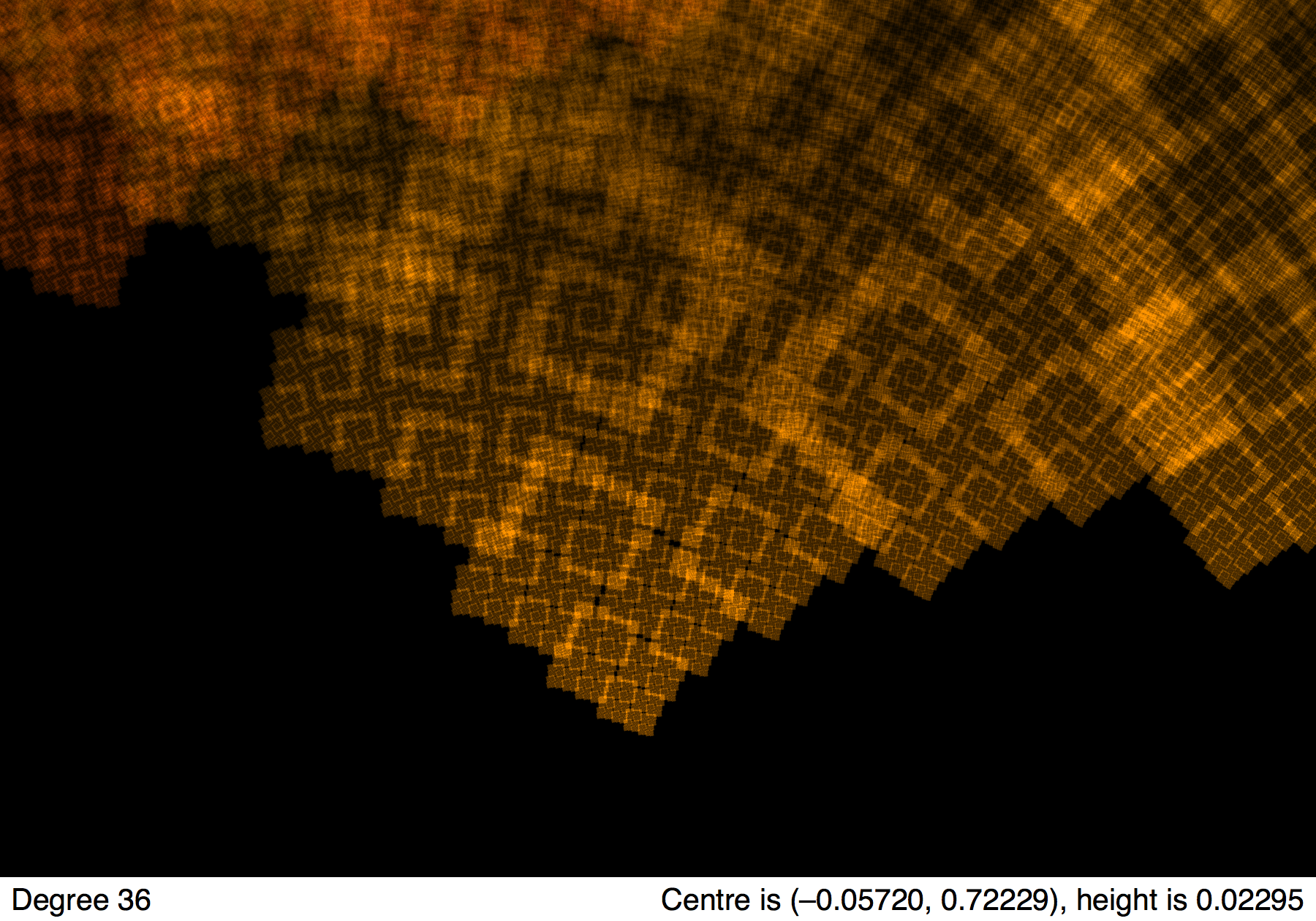
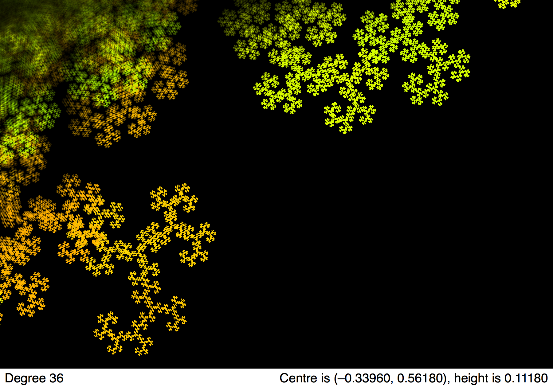
A few sample screenshots from the applet follow:

Here is the full set of roots rendered by the same applet. Unfortunately, computing this kind of view takes too long to be practical for interactive purposes.
