
equation
for r0(r)
In the history of special relativity, numerous thought experiments have involved rotating rings, disks and hoops. One striking feature of a uniformly rotating body in special relativity is that a family of observers who are tied to the body – and hence in a colloquial sense might seem to be “at rest” relative to each other – nonetheless can’t synchronise their clocks, or agree on a shared definition of how spacetime should be split up into space and time. The reason, of course, is that the forces that maintain the body’s shape are accelerating each point of the body, and the magnitude and direction of the acceleration varies from point to point. Unlike the situation where observers are tied to a body undergoing uniform linear motion, there is no way to slice up spacetime into hypersurfaces that are everywhere orthogonal to the observers’ world lines.
The purpose of this web page is to give a very simple model for an annular ring of elastic material rotating with a constant angular velocity in the plane of the ring. If the inner radius of the annulus is zero, we have a disk; if the inner and outer radii are equal, we have a hoop. We will assume that the vertical thickness of the ring is zero, making the problem essentially one in two spatial dimensions, plus time.
Acknowledgement: I wrote this page in response to a discussion on the online Physics Forums, largely between Chris Hillman and a poster going by the name of “Pervect”. It incorporates some of their results and suggestions, but of course any errors here are solely my responsibility.
Caveat: I don’t pretend to be an expert on this subject, and readers should assess everything I’ve written here with care. Also, it’s important to be aware of the limitations of the model.
We will adopt a simple linear model of elasticity appropriate for material under tension: we will assume that, for each infinitesimal element of the body, Hooke’s law will hold exactly. In the context of our two-dimensional problem, what this means is that a small unit square of material which is stretched along either axis will respond with a tension that is proportional to the amount by which its dimension in that direction has been increased. (A discussion of how this model works in special relativity with just one spatial dimension is given in this page on relativistic elasticity.) Although a general deformation in two dimensions can involve shearing — a distortion of the material in which a square becomes a parallelogram rather than a rectangle – this does not arise in the model of the rings we are considering. Also, we will assume that stretching a square in one direction causes a negligible change in its width in the other dimension (in reality most materials will become narrower, a phenomenon quantified by their Poisson’s ratio).
With a rotating ring we will be dealing with a situation where material is stretched, and hence is under tension; however, the conventional way of describing these forces is in terms of pressure, p, so we will follow that and simply be aware that we are dealing with negative values for p. It will also be convenient to talk about a ratio by which the material is compressed in either of two orthogonal directions, which we will describe by the factors ni (with i indexing the two directions), and then keep in mind that our values for ni will be less than 1, and hence describe expansion of the material.
If we take a unit square of material, and deform it into a rectangle of dimensions s1 by s2, then its total potential energy would be:
U = (k/2)[(1–s1)2 + (1–s2)2]
giving rise to forces in the two orthogonal directions of:
f1 = –∂s1U = k (1 – s1)
f2 = –∂s2U = k (1 – s2)
If we rewrite this in terms of ni=1/si, the basic material model becomes:
ε = (k/2) [(1 – 1/n1)2 + (1 – 1/n2)2] n1 n2
p1 = k (1 – 1/n1) n2
p2 = k (1 – 1/n2) n1
Here we’ve taken the total energy and forces associated with an element of the material that is a unit square when undeformed, and multiplied them by the appropriate compression factors, to give ε, the density of potential energy in the material per unit of actual area, and pi, the pressures.
The constant of proportionality, k, is the Young’s modulus for the material. If the rest-mass density of the material in its undeformed state is ρ, it will be useful to introduce the parameters:
K2 = k/(2 ρ)
Q2 = 1 + K2
where K will be the speed of sound in the relaxed (undeformed) material divided by √2, and hence (in units where the speed of light is 1), must satisfy:
K < 1/√2.
This is not the only restriction we need to keep in mind. The weak energy condition requires that the tension in a body does not exceed its energy density (otherwise some observers in motion relative to the body could measure a negative energy density). This can be imposed by the requirement that the factors by which the material is stretched in each direction, si, obey the limit:
si = 1/ni < Q / K
We would also like to restrict the speed of sound to be less than the speed of light in all generality, not just when the material is in its relaxed state. Unfortunately, it is not a trivial matter to calculate the requirements that will guarantee this! For a hyperelastic string held in a straight line under near-uniform tension, it is shown on the accompanying relativistic elasticity page that the speed of sound will reach the speed of light when 1/n = Q/(√3 K), i.e. at a stretch factor some 57% of the maximum imposed by the weak energy condition. The speed at which information is conveyed by vibrations in the rotating bodies we are studying will not necessarily match the speed in a string under identical tension; however, short of a precise formula for the actual speed, we should treat the results we find at similar or higher tensions with a great deal of caution.
We now turn to the question of the world lines of the material of the ring. If we start with cylindrical coordinates (t, r, φ) in 2+1 Minkowski spacetime, in the frame in which the centre of the ring is at rest, we can describe the world line of any particle of the ring by the curve:
(t, r, φ) = (t, r(r0), φ0 + ω t)
where r0 and φ0 refer to the polar coordinates of the particle in the ring in its motionless, unstretched state, and ω is the constant angular velocity of the ring. The function r(r0) that tells us the new radial position of each particle as a function of its initial position is yet to be determined. Discovering the relationship between r and r0 is really the heart of the problem.
From these world lines, we can compute the proper acceleration of each particle; the magnitude of this is:
a(r) = ω2 r / Ω(r)2
where Ω(r) = √ (1 – ω2 r2)
It will be convenient to introduce a field of three orthonormal vectors at each event in spacetime: the timelike vector u pointing along the world line that passes through the event, the radial vector r, and the tangential vector w orthogonal to both u and r. In terms of unit vectors et, er and eφ associated with our cylindrical coordinates, we have:
u = (et + ω r eφ) / Ω(r)
r = er
w = (eφ + ω r et) / Ω(r)
For an observer tied to the material of the ring, u is the direction of time, and r and w are the local directions of space. Note, however, that it’s not possible to join up all the local small planes spanned by r and w at different events, to yield surfaces that are orthogonal everywhere to the world lines of the rotating material.
Given some as-yet-unknown function r(r0) that describes the new radial coordinate of our material, we can determine the ratios nr and nw that describe the deformation. At this point it becomes more convenient to talk about r0 as a function of r, in which case we can write:
nr = r0'(r)
nw = Ω(r) r0(r) / r
In other words, the material is compressed radially by a factor equal to the rate at which its original radial coordinate changes with respect to the new, and compressed tangentially by the ratio of the old radius (and hence arc length) to the new, with a factor to take account of relativistic effects. Specifically, 1/nw is the new spatial distance between the world lines of particles that were originally separated by a unit distance tangentially, so as well as the ratio of circumferences we need to account for the projection of eφ on to w. This means that for a given change in radius, relativistic effects lead to the material being stretched more than in the Newtonian case.
Now that we have the compression ratios, we simply plug those in to our formulas for energy density and pressure. We can then write the stress-energy tensor for the material, which will be:
T = (ε + nr nw ρ) u ⊗ u + pr r ⊗ r + pw w ⊗ w
Conservation of energy-momentum is satisfied in special relativity by requiring that the divergence of this tensor is equal to zero. It’s not too hard to evaluate this divergence. First we note the Leibniz rule for the tensor products we have here:
div (f v ⊗ v) = (v·∇f) v + f (div v) v + f (v·∇) v
All of the scalar functions that appear in T are dependent only on the r coordinate, so we always have:
∇f = (∂r f) r
For our three vector fields, we have:
div u = div w = 0
div r = 1/r
(u·∇) u = – a(r) r
(w·∇) w = – r / (Ω(r)2 r)
(r·∇) r = 0
So we have altogether:
div T = [ – a(r) (ε + nr nw ρ) – pw / (Ω(r)2 r) + ∂rpr + pr / r ] r = 0
We can expand this into a differential equation for our function r0(r):
|
Relativistic equation for r0(r) |
This equation is non-linear, and as far as I know can only be solved numerically. Now, we can extract a Newtonian version of this by setting Ω(r)=1, and also setting terms multiplied by K2 ω2 to zero; this second step is justified because a Newtonian approximation will only be valid when K, which is proportional to the speed of sound, is small. The result is:
 |
Newtonian equation for r0(r) |
We can independently verify this equation as the balance between Newtonian centrifugal force, the tangential tension in the ring, and the rate of change of the radial tension in the ring.
If we prefer to work with r as a function of r0, we can use elementary calculus to re-express these equation in terms of the inverse function:
 |
Relativistic equation for r(r0) |
and the Newtonian version:
 |
Newtonian equation for r(r0) |
These are second-order differential equations, with two-parameter families of solutions, parameterised by the inner and outer radii of the ring. The boundary condition to impose is that the radial tension must vanish at these radii, which means nr = r0'(r) = 1/r'(r0) = 1.
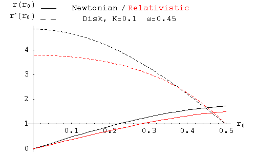
Plotted below are numerical solutions for both the Newtonian and relativistic equations, for a ring with original inner and outer radii of 0.1 and 0.5.

Note that the ring expands more in the Newtonian case than in the relativistic case. Below is a plot for a disk of original radius 0.5.
In the case of a “hoop”, where we take the limit as the inner and outer radii of a ring approach the same value, we can replace our differential equations with simpler equations relating the single values for the original and rotating radii, r0 and r. To make this transformation, we assume that r'(r0), rather than crossing the value of 1 at two distinct radii, reaches a maximum value of 1 at a single radius, that of the hoop. Because r'(r0) lies at an extremum, r''(r0)=0. So we can simply substitute r'(r0)=1 and r''(r0)=0 into our differential equations. The result in the relativistic case is:
ω2 Ω(r)2 r r02 + 2 (K/Q)2 Ω(r)3 r0 – (K/Q)2 (Ω(r)2 + 1) r = 0
where Q2 = 1 + K2
This is messy to solve explicitly for r in terms of r0, though it can be rearranged into a cubic in r2, so it can be solved analytically. For r0 in terms of r, it is simply a quadratic.
| r0 = K [ –K Ω(r)2 + √(Q2 – Ω(r)4) ] / [ Q2 Ω(r) ω2 r ] | Relativistic hoop equation for r0(r) |
It’s also possible to express r and ω in terms of nw, parameterising the solution according to the compression factor for the hoop, which will lie between a minimum value of K/Q, set by the weak energy condition, and 1. (A poster on the online Physics Forums going by the name “Pervect” discovered this parameterisation).
| r = (r0 / nw) √[ (1 – Q2 (1 – nw2)) / (nw2 + K2 (1 – nw)2) ] | Relativistic hoop equation parameterised by nw |
| ω = (K nw / r0) √[ 2 (1 – nw) / (1 – Q2 (1 – nw2)) ] |
The Newtonian case gives us:
ω2 r r02 = 2 K2 (r – r0)
This makes perfect sense, because it is really just expressing the balance between centrifugal force and tension for an element of the hoop; with a little rearrangement, it can be seen to be equivalent to:
(ρ r0 dφ) ω2 r = k (r/r0 – 1) dφ
The Newtonian equation is easily solved for either variable:
| r0 = K [ –K + √(K2 + 2ω2 r2) ] / [ ω2 r ] | Newtonian hoop equation for r0(r) |
| r = 2 K2 r0 / (2 K2 – ω2 r02) | Newtonian hoop equation for r(r0) |
In the second Newtonian equation, as ω r0 approaches the speed of sound in the relaxed material, K √2, the denominator approaches zero, so this sets a ceiling on the angular velocity for a hoop in equilibrium.
The plot below shows r vs r0 for a fixed K and ω. In the Newtonian case, the radius of the spinning hoop goes to infinity as r0 approaches the critical value K √2 / ω. In the relativistic case, r is constrained by the need to keep ω r < 1. Eventually this means that a large enough hoop spun up to this angular velocity must shrink; this occurs after the red curve crosses the dashed line r=r0.

The next plot is for a hoop of initial radius r0=1, at various values of ω. The dashed curves give the tension in the hoop (divided by 2k for convenience, in order to fit the same scale as r), as measured locally in the material’s rest frame. In other words, this is the tension that the material “experiences”.
The radius for the Newtonian case goes to infinity as ω approaches K √2 / r0. In the relativistic case, r reaches a maximum and then declines. Note, however, that the tension in the hoop continues to increase even as the radius measured in the Minkowski frame shrinks, because relativistic effects allow the material to continue to expand.
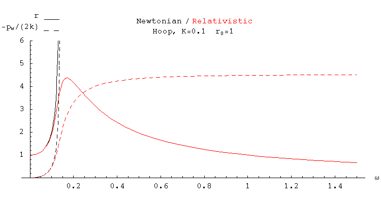
The tension approaches a horizontal asymptote (–pw/k → Q/K–1) as ω goes to infinity and r approaches zero. This asymptote coincides with the point where the tension would violate the weak energy condition; any real material would break somewhere before this point, imposing a finite maximum on the possible value ω can reach.
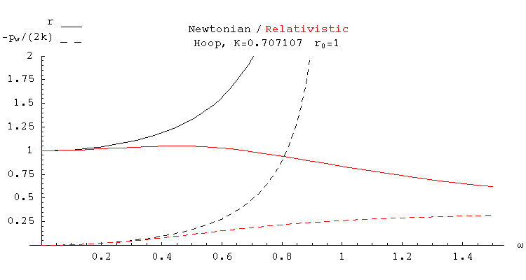
Below, the radius and tension are plotted for a maximally stiff material, in which the speed of sound equals the speed of light.
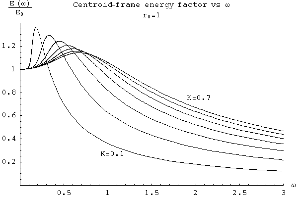
By integrating Ttt, the energy density in the Minkowski frame in which the centroid of the hoop is at rest, we can derive a total energy for the rotating hoop. We express this as a ratio with E0, which is just the total rest mass of the stationary hoop, in terms of the parameter nw. We have already expressed r and ω in terms of the parameter nw, here.
| E(ω) / E0 = (Q2 nw + K2 (3 / nw – 4)) r / r0 | Centroid-frame energy factor (hoop in equilibrium) |
The plot below shows this energy factor across a range of angular velocities, and for a selection of K values. In all cases, the energy rises to a maximum and then falls. This is the result of an interplay between two competing effects: the rise and fall of the hoop’s radius, and the fall and rise of the energy density measured in the centroid frame. (The energy density initially falls simply because the hoop is expanding under centrifugal force, diluting the density of its rest mass; later, things become more complicated, with potential energy driving it up, Lorentz-mixing with tension driving it down, and a relativistic factor of 1/Ω(r)2 driving it up.)
Eventually the total energy drops below the initial rest-mass energy! In other words, an elastic hoop rotating with sufficient angular velocity (albeit one with a spectacularly unlikely breaking strain) would seem to have a form of “binding energy” in the centroid frame greater than its kinetic energy.
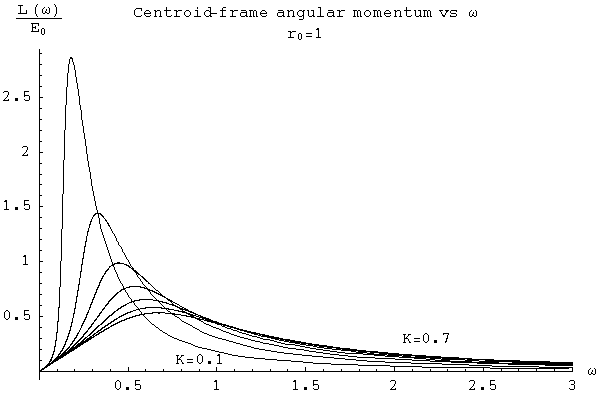
The angular momentum also rises to a maximum and then falls.
| L(ω) = E(ω) ω r2 / (1 + ω2 r2) | Centroid-frame angular momentum (hoop in equilibrium) |
My first response when I calculated the energy curve was “This can’t be true! What happens if you lower the energy of a hoop below its rest mass, and then it breaks? Where does the energy come from for the fragments to exist in a normal, tension-free state?” The answer is two-fold. Firstly, the idealised hyperelastic material simply can’t break, so if you stick to that model the issue never arises. Secondly – and more realistically – if you switch to a material model with a different potential energy curve which allows the tension to drop off and eventually go to zero when you stretch the hoop too far, what happens is that the total energy curve changes: once the tension stops growing, the energy stops falling, and by the time the tension hits zero the total energy will be above the rest mass again. So for a breakable hoop, in order to actually break it you will need to put in enough energy to bring it back above its rest mass.
However, although that initial paradox proved unfounded, we need to be cautious. The plot below shows the value of nw where the peaks in the radius and the energy occur, along with the values where the weak energy condition is violated, and where the speed of sound in a linear string will reach the speed of light. The fact that the hoop needs to be stretched beyond the point where the speed of sound in the same material hits c (albeit in a different physical configuration), shows that (at the very least) we’re pushing close to the model’s limitations here.
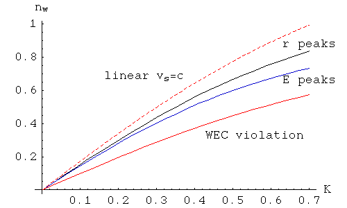
Later, we’ll see that there definitely are some serious problems that occur before we reach the energy peak.
In our online discussion, the question arose as to whether a rotating hoop would be stable. We know that we’ve found equilibrium solutions for a range of perfectly axially symmetric hoops, but can we trust our intuition which says that a taut string will snap back into place from any small deformation? Note that we are using the word “hoop” here to describe what is essentially a 1-dimensional string, which offers no resistance to bending. We are not considering something like a metal hoop with a small but finite width that will resist bending.
We will analyse two classes of deformation: pulsations, where the hoop’s radius is perturbed slightly while retaining axial symmetry, and vibrations, where we will look for waves similar to those of a plucked string. If the hoop is in a stable equilibrium, such small deformations should attract counteracting forces that lead to simple harmonic motion; if the hoop is in an unstable equilibrium, the deformations will instead grow exponentially.
We will start by investigating the simplest case, the pulsations of a Newtonian hoop.
The most straightforward way to analyse a pulsation – where we perturb the radius of a hoop away from its equilibrium value without distorting its shape — is very similar to a standard technique for analysing planetary orbits. In Newtonian planetary orbits, the potential energy due to gravity forms a “funnel” shape that grows negative as 1/r, but centrifugal force effectively adds a countervailing “chimney”, that grows positive like 1/r2. Adding the two produces an energy “trough” around the central object, at the very bottom of which lies the circular orbit for a given amount of angular momentum:
 |
+ |  |
= |  |
| Gravitational potential | Centrifugal “potential” | Combined “potential” |
|---|
What we’re doing in such an analysis is looking at how the total energy of a system changes with r as we move away from a given equilibrium state, while imposing the constraint of conservation of angular momentum. So to examine pulsations of a hoop, we will need to know the total energy of hoops with radii close to our equilibrium hoop, with exactly the same angular momentum. These neighbouring hoops will not be in equilibrium themselves, but we will compute their energy for the situation when their radius is instantaneously unchanging. The idea is that if we find our equilibrium hoop to lie at the bottom of an energy trough or valley compared to these neighbours, then it would use up the energy in any small radial motion we gave it to climb a short way up the sides of the valley, and end up oscillating within the valley. However, if we find our equilibrium hoop on the top of an energy ridge, then there will be nothing to contain it from continuing to move in the direction of any small push.
More formally, we want to know if the second derivative of the energy of a hoop with respect to r, evaluated with the constraint of constant angular momentum, is positive (stable equilibrium) or negative (unstable equilibrium).
The total angular momentum of a perfectly circular Newtonian hoop, with relaxed radius r0, relaxed linear density ρ, current radius r, and angular velocity ω, is:
L = M ω r2
where M = 2 π ρ r0 is the total mass of the hoop. The total energy, the sum of kinetic and potential energy (for a hoop whose radius is instantaneously unchanging), is:
E = (1/2) M ω2 r2 + π k r0 (r/r0 – 1)2 = (1/2) M ω2 r2 + M K2 (r/r0 – 1)2
If we express ω in terms of L, and substitute that into our formula for E, we have:
ω = L / (M r2)
E = L2 / (2 M r2) + M K2 (r/r0 – 1)2
dE / dr = – L2 / (M r3) + 2 M K2 (r/r0 – 1) / r0
d2E / dr2 = 3 L2 / (M r4) + 2 M K2 / r02 = M (3 ω2 + 2 K2 / r02)
The second derivative is clearly positive everywhere. If we substitute the equilibrium value for r:
req = 2 K2 r0 / (2 K2 – ωeq2 r02)
into these formulas, we get:
dE/dr|eq = 0
d2E / dr2|eq = M (3 ωeq2 + 2 K2 / r02)
Now, what this tells us is that, given the constraint of conservation of angular momentum, near the equilibrium the radial degree of freedom has associated with it an effective “potential energy” Ueff(r) (which really consists of both elastic energy and rotational kinetic energy) that takes the form of a simple harmonic oscillator’s potential:
Ueff(r) = (1/2) (d2E / dr2|eq) (r – req)2
So small pulsations in r will take the form:
r(t) = req + A cos(ωpulse t)
where ωpulse2 = 3 ωeq2 + ωc2
and we have made use of the critical angular velocity, ωc, which the hoop cannot exceed:
ωc = K √2 / r0
As r pulses back and forth around the equilibrium value, ω will also rise and fall, to conserve angular momentum:
ω(t) = ωeq (req / r(t))2
To analyse the stability of small pulsations of a relativistic hoop, we apply the same basic ideas as we’ve used for the Newtonian case. We find the total energy and angular momentum of a hoop by integrating Ttt and r Ttφ respectively. The results are simpler if we make use of the parameter:
s = 1/nw = r / (r0 √ (1 – ω2 r2))
which measures how much the hoop has been stretched. Because we know that r reaches a maximum and then falls as the angular velocity increases, it will be convenient to use s rather than r as our degree of freedom, since s grows monotonically with ω. We’ll also define two useful abbreviations:
s1 = 1 – K2 (s2 – 1)
s2 = 1 + K2 (s – 1)2
Note that 1≤s<Q/K, where Q=1+K2, and that both s1 and s2 will be positive within this domain for s. In terms of s and ω we then have:
L = M r02 s1 s2 ω / √(1 + r02 s2 ω2)
E = M (r02 s1 s2 ω2 + s2) / √(1 + r02 s2 ω2)
In principle we could solve for ω as a function of L and substitute the result into E, but we can avoid the messy algebra that would entail by using the requirement for L to be constant to find the value of dω/ds, which we can then employ in the derivatives of E. We find that dL/ds=0 implies:
dω/ds = (ω / (s s1)) [r02 s2 ω2 (2 Q2 – 3 s1) + 2 Q2 – 4 s1]
which then allows us to write:
dE/ds = M [s2 (Q2 – 3 K2 s2) ω2 r02 + s1] [2 K2 (s – 1) – s ω2 r02 s1] / [s1 √(1 + r02 s2 ω2)]
This will be zero when ω=ωeq:
ωeq = (K / r0) √(2 (s – 1) / (s s1))
which is identical to the solution for the equilibrium we previously expressed in terms of nw. If we evaluate the second derivative and then set ω to ωeq, we find:
d2E/ds2|eq = 2 M K2 p(s) q(s) / (s √(s17 s2))
p(s) = 6 K4 s5 – 19 K4 s4 + 6 K2 (3 K2 + 1) s3 – 4 Q2 (2 K2 + 1) s + 3 Q4
q(s) = 5 K4 s4 – 6 K4 s3 + 2 Q2 K2 s – Q4
The polynomial p(s) turns out to be equal to an always-negative multiple of the derivative of the total energy of an equilibrium hoop with respect to s. So p(s) will be negative when the hoop is less stretched than it is at its energy peak, and positive after that. In fact, p(1)=q(1)=–1, so both polynomials are initially negative, while both are positive at the maximum value for s, Q/K. Numerical calculations show that for the range of admissible values of K, both polynomials have a single zero in the domain for s, with the zero of q(s) always less than that of p(s). For example, for K=0.1, q(6.80411)=0, p(6.89933)=0, and for K=0.7, q(1.31214)=0, p(1.36355)=0.
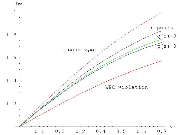
The plot below shows the points where q(s)=0 for a range of K values, along with various other features we’ve shown before; p(s)=0 is where the energy peak occurs. The vertical axis here is nw, the compression factor, so the lower a curve the greater the degree of stretching it describes.
In all cases there is a range of values for s where p(s) and q(s) have opposite signs, resulting in an unstable equilibrium. Nevertheless, it looks as if this instability can’t lead to run-away behaviour, because the energy ridge on which it occurs is contained on both sides by a deeper valley. The plot below illustrates this for K=0.1; this curve was plotted by first computing L for the point of unstable equilibrium, then solving for ω as a function of s while keeping L fixed at that value, and inserting the result into the formula for E.

How far can we trust these results? The verdict that the relativistic hoop will be stable against pulsations for low values of the stretch factor s is probably reliable, but we will see later that when s crosses the zero of q(s), the hyperelastic model shows signs of becoming completely unphysical.
Having dealt with pulsations, in which the hoop’s radius oscillated while its circular shape was maintained, we will now consider vibrations in which its shape becomes slightly distorted, while its average radius remains fixed. For example, we can imagine sinusoidal waves, either transverse to the hoop (local changes in the radius) or longitudinal (local changes in the degree of stretching). However, it turns out that the rotation of the hoop demands that both modes, transverse and longitudinal, occur together. If a small segment of the hoop is deflected out to a greater radius, it’s no use simply appealing to overall conservation of angular momentum and saying that another small segment elsewhere balances this by moving inwards; local conservation of tangential momentum means that the segment will trigger a longitudinal elastic response as it attempts to reduce its angular velocity.
We will look for small-amplitude vibrations such that the polar coordinates of the material of the hoop take the form:
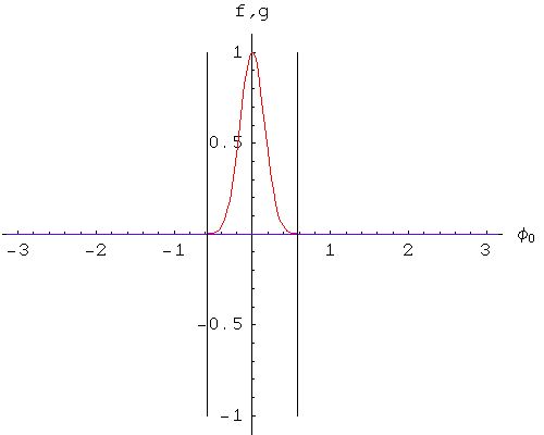
r(t, φ0) = req + f(t, φ0)
φ(t, φ0) = φ0 + ω t + g(t, φ0) / req
where it is assumed that f and g and all their derivatives up to second order are small. We will work in a rotating orthonormal basis {er, eφ}, whose basis vectors are functions of both time, t, and φ0, which identifies the particular piece of hoop material we’re looking at.
er = cos(φ0 + ω t) ex + sin(φ0 + ω t) ey
eφ = –sin(φ0 + ω t) ex + cos(φ0 + ω t) ey
∂ter = ω eφ
∂teφ = –ω er
∂φ0er = eφ
∂φ0eφ = –er
We can write the location of a particle of the hoop with original angular coordinate φ0, at time t, as:
x(t, φ0) = (req + f(t, φ0)) er + g(t, φ0) eφ
where we have made use of the small amplitude of f and g to give a linear expression. It’s then straightforward to compute the acceleration:
a(t, φ0) = (∂t,tf – ω2(req + f) – 2 ω ∂tg) er + (∂t,tg – ω2g + 2 ω ∂tf) eφ
Here the second rates of change with time of f and g are simply augmented by the centripetal and Coriolis accelerations in the usual way.
Next we compute the vector equal to the rate of change of x with respect to unstretched length; we will call this t because it is a tangent to the hoop:
t(t, φ0) = (1/r0) ∂φ0x(t, φ0) = (1/r0)[ (∂φ0f – g) er + (req + f + ∂φ0g) eφ]
From this, we compute the tension vector S to first order:
S(t, φ0) = k (|t|–1) t/|t| = (k/r0)[ (1 – r0/req)(∂φ0f – g) er + (req– r0 + f + ∂φ0g) eφ ]
In earlier versions of this page (prior to 20 June 2007) I assumed that the tension in the hoop, |S|, could be treated as constant, because any variation would be lower than first order. Although that assumption is correct for small waves in a straight string, for a hoop it is only correct for a certain class of solutions, not all of them!
From S we obtain the force F per unit of unstretched length:
F(t, φ0) = (1/r0) ∂φ0S(t, φ0)
= (k/r02)[ (–f – (2 – r0/req) ∂φ0g + (1 – r0/req) (∂φ0,φ0f – req)) er + (–(1 – r0/req) g + (2 – r0/req) ∂φ0f + ∂φ0,φ0g) eφ ]
Equating this to ρ a(t, φ0), the two components give us two coupled linear partial differential equations:
 |
PDEs for Newtonian hoop vibrations |
Here we have re-expressed req in terms of the critical angular velocity ωc:
ωc = K √2 / r0
req/r0 = ωc2 / (ωc2 – ω2)
1 – r0/req = ω2 / ωc2
We will now look for harmonic solutions of the form:
f(t, φ0) = δ cos(m(φ0– c ω t))
g(t, φ0) = δ α sin(m(φ0– c ω t))
so that:
r(t, φ0) = req + δ cos(m(φ0– c ω t))
φ(t, φ0) = φ0 + ω t + δ (α / req) sin(m(φ0– c ω t))
where δ is much smaller than req. The parameter m will be a non-zero integer, in order for the wave to be continuous at φ0 = 2π; c determines the angular velocity of the wave relative to the material, and α determines the amplitude of the longitudinal wave compared to that of the transverse wave.
If we substitute the trigonometric functions here for f and g into our PDEs, we get two polynomial equations in c and α. The polynomial from the second of the PDEs is linear in α, giving:
α = [(2 c + 1) ω2 + ωc2] / [m (c2 ω2 – ωc2)]
Substituting that into the polynomial from the first PDE gives the equation:
(c + 1) (m2 c3 – m2 c2 – (3 + (m2 + 1) ωc2 / ω2) c + (m2 – 3) ωc2 / ω2 – 1) = 0
This gives one obvious, simple class of solutions, where c = –1 and α = –1/m. Since these waves are travelling in the material of the hoop with an angular velocity exactly opposite that of the rotation, in the stationary centroid frame they will appear as deformations that are almost fixed in space; however, the longitudinal vibration will cause the shape to fluctuate slightly, with only the extrema of the transverse radial waves – corresponding to nodes in the longitudinal waves – being perfectly fixed.
These c = –1 sin/cos solutions generalise to travelling waves of the same velocity of arbitrary shape:
f(t, φ0) = –G'(φ0 + ω t)
g(t, φ0) = G(φ0 + ω t)
where of course we need G to be twice-differentiable and periodic with a period of 2π.
There are other sin/cos travelling wave solutions, which come from the roots of the cubic in c. We first note that changing the sign of m reverses the sign of α but has no effect on c, so because of the way sin and cos transform under a change of sign of their argument there is no net effect on the solution at all.
For m=1 the cubic factors into (c + 1), for a solution we’ve already seen, and a quadratic with two real roots:
c = 1 ± √(2 [1 + ωc2 / ω2])
both of which give α = 1. Note that the m=1, c=–1 solution simply represents a translation of the hoop, not a change in its shape. What’s more, the same solutions for f and g multiplied by t will also solve the partial differential equations; this represents the hoop’s centre-of-mass undergoing inertial motion.
For higher values of m, the cubic term will again have three real roots. How can we be sure of this? If we call the value of the cubic C(c), then:
So C(c) changes sign three times, and must have three real roots. Because the velocities of these waves depend on m, which determines the wavelength, these solutions are dispersive; waveforms that contain multiple wavelengths will change shape as they propagate. The angular velocity of these waves is plotted below, for m ranging from 1 to 5 and for ω ranging from 0 to ωc; here it has been re-expressed more conveniently as a fraction of ωc.

In the limit where ω → ωc, the cubic factors to give the simple rational solutions c = –1, c = (m+2)/m, and c = (m–2)/m. This represents the high-tension limit, where the angular velocity is close to the critical value and the equilibrium radius is much greater than the relaxed radius. At the other extreme, ω → 0, the corresponding limits of cω/ωc are –√(1+1/m2), √(1+1/m2) and 0; in the first two cases c itself goes to infinity, while in the last it tends towards the finite value (m2–3)/(m2+1).
A third limit we can take is m → ∞, in which case the three solutions tend to c=–ωc/ω, c=ωc/ω, and c=1. This needs to be interpreted carefully, because if we let m go to infinity while holding δ fixed, a high enough value for m will eventually contradict the assumption that our perturbation’s derivatives are small, and we will not be justified in using the linearised PDEs. Nevertheless, we note that the linear velocity, r c ω, associated with the largest of these angular velocities is simply (r/r0) K √2, which is the speed of sound in a string stretched by a factor of (r/r0); in other words, in the short-wavelength limit the fastest vibrations in the hoop (which as we’ll see below are purely longitudinal) propagate as they would in an equally stretched straight string.
The ratio of the amplitude of the longitudinal vibrations to that of the transverse, α, is plotted below for the same range of values for m and ω. Note that as ω → ωc, one solution for α goes to infinity (unless m=1), while the other two go to 1 and –1. As ω → 0, the first two solutions go to m, while the third goes to –1/m. And as m goes to infinity, the first two solutions for α go to infinity (purely longitudinal waves), while the third goes to zero (purely transverse waves).

Examples of all of these waves can be seen in the numerical simulation performed by the Newtonian hoop applet.
Finally, we note that these differential equations yield a result that agrees with our earlier analysis of pulsations. If we look for axially symmetric solutions of the form:
f(t) = δ cos(ωpulse t)
g(t) = δ α sin(ωpulse t)
then we find ωpulse = √(3ω2 + ωc2), α = –2ω/ωpulse. This agrees with our previous formula for the frequency of pulsations.
To analyse vibrations of a relativistic hoop, we need to construct an appropriate stress-energy tensor for a hoop undergoing a more general motion than rotating at a constant angular velocity with a fixed radius and a perfectly circular shape. In terms of three orthonormal vector fields – u, tangent to the world lines of the hoop material, w, tangent to the world sheet of the hoop and orthogonal to u, and r, orthogonal to both u and w — we have:
T = ρ(s) u ⊗ u + P(s) w ⊗ w
where
ρ(s) = [ ρ + (k/2) (1–s)2 ] / s
P(s) = k (1–s)
and s is the stretch factor, 1/n. Setting the divergence of T to zero yields:
∇wP(s) + (ρ(s) + P(s)) (w·a) = 0
P(s) r.(∇ww) + ρ(s) (r·a) = 0
where a = ∇uu
These equations make sense in an almost “F=ma” way: the first says that spatial changes in the pressure give rise to an acceleration of material tangential to the world sheet, albeit with an effective mass of (ρ(s) + P(s)) that is made less by the presence of tension. The second says that the combination of pressure and any curvature of the world sheet (any turning of its spatial tangent w) give rise to an acceleration of material normal to the world sheet.
These equations can be expressed as two non-linear partial differential equations for functions r(t, φ0) and φ(t, φ0) that describe the world sheet of the hoop. We then assume a small deviation from equilibrium of the form:
r(t, φ0) = req + f(t, φ0)
φ(t, φ0) = φ0 + ω t + g(t, φ0) / req
Taking quantities to first order in f and g, we obtain two linear PDEs:
 |
PDEs for relativistic hoop vibrations |
Here n is the compression factor for the equilibrium hoop that we are perturbing, and we have defined abbreviations for two functions of n:
λ2 = n2 + K2 (1–n)2
μ2 = n2 – K2 (1–n2)
Before considering vibrations of the hoop, let’s see what we can find out from these equations about pulsations of the hoop, and compare it with our previous analysis. If we look for axially symmetric solutions of the form:
f(t) = δ cos(ωpulse t)
g(t) = δ α sin(ωpulse t)
then the PDEs yield a quadratic in ωpulse:
r02 s s1 (3 K2 s2 – 4 K2 s + Q2) q(s) ωpulse2 = 2 K2 s2 p(s)
where we have switched from the compression factor, n, to the stretch factor, s=1/n, and we are using the same abbreviations as in our previous analysis of pulsations:
s1 = 1 – K2 (s2 – 1)
s2 = 1 + K2 (s – 1)2
p(s) = 6 K4 s5 – 19 K4 s4 + 6 K2 (3 K2 + 1) s3 – 4 Q2 (2 K2 + 1) s + 3 Q4
q(s) = 5 K4 s4 – 6 K4 s3 + 2 Q2 K2 s – Q4
Apart from p(s) and q(s) the other terms in the quadratic for ωpulse are positive for 1<s<Q/K, so as before we find that we will have stable pulsations when the signs of p(s) and q(s) agree. We won’t give the corresponding solution for α, but we note that it goes to infinity when p(s) or q(s) are zero, while it is equal to zero when the equilibrium radius of the hoop is at its maximum. In other words, pulsations of the hoop around the maximum equilibrium radius take place without any change in angular velocity; this is also the point where the derivative of the angular momentum of the hoop with respect to the radius is zero.
Later, we will be interested in describing vibrations of the hoop with arbitrary initial conditions for f, g and their time derivatives. If we perform a Fourier analysis of those four initial conditions, matching the constant terms (those with no angular dependence) will require four independent axially symmetric solutions of our PDEs. We have seen one solution; what are the rest? The second solution comes from swapping cos and –sin (or equivalently, taking the derivative with respect to t) of the first solution. The third comes from setting f(t) to zero, and g(t) to any constant; this represents rotating our polar coordinate system by some constant amount. The fourth comes from setting f(t) to a constant, and making g(t) linear in t; this represents simply shifting the hoop to a new equilibrium, with a new radius and new angular velocity.
Next we look for harmonic solutions of the form:
f(t, φ0) = δ cos(m(φ0– c ω t))
g(t, φ0) = δ α sin(m(φ0– c ω t))
as we did for the Newtonian case. Again, this yields two polynomial equations in c and α. The solution for alpha in terms of c is:
 |
Relativistic alpha |
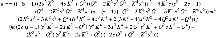
When we eliminate α, the polynomial in c we obtain has a factor of (c+1) and a cubic term. As in the Newtonian case, c=–1 implies α=–1/m, so the c=–1 solutions are unchanged in the relativistic case. The cubic in c, however, is much more complicated:
 |
Relativistic cubic in c |
As in the Newtonian case, for m=1 this cubic has a factor of (c+1), giving the root c=–1 a second time, and leading to solutions representing translation and inertial motion of the hoop’s centre of mass, rather than any change of shape. In the Newtonian case, the second m=1, c=–1 solution (for inertial motion) was simply t times the first solution; in the relativistic case there’s an extra term in the longitudinal wave:
f(t, φ0) = δ t cos(φ0+ ω t)
g(t, φ0) = – δ t sin(φ0+ ω t) – δ req2ω cos(φ0+ ω t)
Altogether, for each value of m we have a total of eight solutions, with four where f is a cosine and four where f is a sine. For each set of four, in general c takes the values –1 and the roots of the cubic, while for m=1, there is a special pair of solutions for the double root c=–1. Along with the four axially symmetric solutions we described previously, these solutions allows us to match the cosine, sine and constant Fourier components of arbitrary initial conditions for f, g and their time derivatives.
Eagle-eyed readers might have noticed that one of the factors of the leading coefficient of the cubic is none other than the polynomial q(s), whose zeroes mark the onset of instability in axially symmetric pulsations. It turns out that the same values for s mark a blow-up in the roots of the cubic. Plotted below are the phase velocities corresponding to the three roots, for m ranging from 1 (red curves) to 5 (magenta curves), as well as the limiting value as m goes to infinity (black curves). These are shown as linear velocities in the non-rotating centroid frame; we add one to c because even a c=0 wave will be moving with the hoop.

It’s apparent that some of these phase velocities are superluminal for much of the range for s; however, that in itself need not be unphysical, as information generally will not travel at the phase velocity when that velocity is dependent on the wavelength. One common means of computing the speed of information flow is to take the limit of the phase velocity as the spatial frequency goes to infinity, the idea being that the leading edge of any initially sharp pulse, such as a step function, would be limited by that speed. Of course, as m goes to infinity the derivatives of the corresponding Fourier components cease to be small, so we need to be careful how we interpret these results.
In the high m limit, the cubic in c factors into a linear term and a quadratic, and it turns out that when s = Q/(√3 K), the roots of the quadratic yield linear velocities of ±1. In other words, when the speed of sound in a straight string reaches the speed of light, the fastest vibrations in the hoop, in the short-wavelength limit, also reach the speed of light.
How clear is it that the hyperelastic model would actually require superluminal signal transmission for high enough stretch factors? The movie below shows an initial square-wave pulse in f propagating through a hoop with K=1/2 and s=1.5; the initial conditions for the pulse were synthesised with Fourier components up to m=100. The moving black lines mark the fastest phase velocities in the short-wavelength limit, and it’s clear that they track the spread of the disturbance reasonably well.

A square wave pulse does not have bounded derivatives, though, so we are not really justified in using the linearised PDEs for that case. The next movie shows a smoother pulse with a bounded second derivative. Here, it’s somewhat less clear whether the disturbance really is spreading at exactly the short-wavelength limit, but what is clear is that the speed of information propagation is not a great deal slower than that. So, while this analysis doesn’t let us pinpoint the onset of superluminal signalling precisely, it suggests that it will occur not long after s = Q/(√3 K). Presumably, this means that any detailed material model consistent with special relativity will necessarily depart from the hyperelastic model before that point.
Finally we note that, unlike the Newtonian case, there are situations where some solutions of the cubic are complex-valued. If we take a conjugate pair of complex solutions for c, and sum the functions to which they correspond, the resulting solutions of the PDE are real-valued functions that grow exponentially with time. In other words, these complex roots identify situations where the shape of the hoop is unstable to small perturbations. The range of values for s where complex values of c appear depends on K and m; we plot one example below.
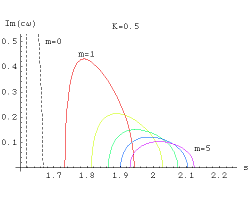
Here the dashed curve labelled m=0 is based on our analysis of axially-symmetric pulsations. The leftmost point of this curve is where q(s)=0; the rightmost point is where p(s)=0, and the energy of the equilibrium hoop reaches its maximum.
So far, we have looked at equilibrium states of the hoop, and also infinitesimal perturbations away from equilibrium. It’s not too difficult, mathematically, to analyse finite pulsations of the hoop; however, we will find that our model becomes completely unphysical at a certain threshold which we’ve seen hinted at in our previous calculations.
We can derive equations of motion for a pulsating hoop by computing the stress-energy tensor of a radially symmetric hoop with a changing radius, and setting the divergence to zero. This is equivalent to setting the rate of change of the total energy and total angular momentum of such a hoop to zero. The energy and angular momentum, divided by the hoop’s rest mass M, are:
E/M = [r02 β1/2 σ + K2 ((r2 + r02) β3/2 – 2 r r0 σ3/2 – r2 (2 r2 + r02) β1/2 ω2)] / [r02 β1/2 σ3/2]
L/M = r2 ω [r02 σ + K2 (r02 β – r2 (β + r02 ω2))] / [r02 σ3/2]
β = 1 – vr2
σ = 1 – ω2 r2 – vr2
where vr is the rate of change of the hoop’s radius, r, with respect to time measured in the Minkowski frame of the hoop’s centre of mass. E and L will be conserved if the radial and angular accelerations ar and aφ – the rates of change in the centroid frame of vr and ω respectively – are given by:
ar = [–2 K2 r0 β σ3/2 + r β1/2 (2 K2 β2 – z1 β ω2 + Q2 r2 r02 ω4)] / [2 K2 r r0 σ3/2 – β1/2 (z1 σ – K2 r4 ω2)]
aφ = 2 vr ω [(–(Q4 r04 β3/2 σ2) + K2 Q2 r r02 σ (2 r β5/2 + r0 σ5/2 + 2 r3 β3/2 ω2) + K4 r3 β (r β5/2 – 3 r0 σ5/2 – 6 r3 β3/2 ω2 + 2 r5 β1/2 ω4))] / [r β (z2 β + r2 (K2 r2 + z1) ω2) (2 K2 r r0 σ3/2 – β1/2 (z1 σ – K2 r4 ω2))]
z1 = K2 r2 + Q2 r02
z2 = K2 r2 – Q2 r02
The problem with the model appears at points where a factor in the denominator of the angular acceleration:
(z2 β + r2 (K2 r2 + z1) ω2)
is zero, and the numerator is non-zero. The result is that the equations of motion here have no solution! This coincides with the derivative of L with respect to ω being zero.
If we look for the conditions when this expression is zero while the hoop is in equilibrium, it turns out that this corresponds precisely to q(s)=0, the point where we have seen a blow-up in the phase velocity of vibrations of the hoop. Of course if the hoop is in equilibrium, then vr is zero, and we can obtain a valid solution to the equations of motion by setting the angular acceleration to zero. But any small perturbation away from the equilibrium here will result in the singular behaviour we’ve described.
Another way to view the problem is to look at the sets in (ω, r, vr)-space that are produced by fixing the values of E and L. The easiest way to study these sets is to parameterise them by s, the factor by which the hoop has been stretched.
r = √[r02 s2 (1 – K2 (s2–1))2 – (L/M)2] / [1 – K2 (s2–1)]
β = 1 – vr2 = [r02 s + K2 (s–1) (2 r2 – r02 s (s+1))] / [(E/M) r r0]
ω = √[β (r02 s2 – r2)] / [r r0 s]
These formulas effectively specify all three coordinates solely in terms of s. The domain for s will consist of either one or two intervals, comprising those values where 0<β≤1 and r and ω are real; we also require 0 < s < Q/K, but that follows anyway from the requirement that r be real. It turns out that the endpoints of the intervals are points where β=1, i.e. vr=0.
When E and L specify an equilibrium configuration, the set in (ω, r, vr)-space will consist of just two discrete points: one for the low-ω equilibrium, and another for the high-ω equilibrium of the same energy. Moving away from the equilibrium, the two discrete points will, generally, grow into two loops (corresponding to two disjoint intervals in the domain for s); the state of the hoop will lie on a particular loop, and will cycle around it. Crucially, r and ω will both be monotonic functions of s when confined to a single interval within the domain, and both will reach their maxima and minima at the endpoints of the interval, where vr=0, allowing the hoop to reverse its radial motion.
However, there are values of E and L where the set in (ω, r, vr)-space consists of a single loop. In those cases, r will reach a maximum value in the interior of the single interval that comprises the domain for s, at a point where vr is non-zero. When the hoop arrives at that state with a positive vr, logically r must keep increasing, but there are no more values for r available such that E and L continue to be conserved.