
What can the elliptical orbits of planets tell us about the energy levels of an atom? An atom isn’t really much like a miniature solar system, but the electrostatic force does obey the same kind of inverse-square law as Newtonian gravity. In the simplest case – a hydrogen atom, with just one proton and one electron – a special symmetry shared by all inverse-square laws leaves a clear mark on the quantum-mechanical version of the system. This has been known since the pioneering days of quantum mechanics, when Wolfgang Pauli used it to compute the energy levels of hydrogen.[1][2] And as we’ll see, this symmetry involves rotations in four dimensions.
In what follows, we’ll take two well-known facts for granted: that the orbit of a single planet around a star under Newtonian gravity is an ellipse (with a circle as a special case), and that the sum of the distances from the two foci of an ellipse to any point on the ellipse itself is a constant. You can find proofs of both these claims here.
We’ll start by considering a planet in a circular orbit around the sun. Of course in reality the planet and the sun would both orbit their common centre of mass, but that doesn’t really change anything important. If we want to take account of it, we can replace the planet’s mass with its “reduced mass”, and then the calculations proceed in exactly the same fashion.
The planet’s velocity vector will change direction as it moves around the orbit, but the planet’s speed – the length of the velocity vector – will remain the same. So if we draw all the velocity vectors from around the orbit with their bases at a common origin, they will form a circle.
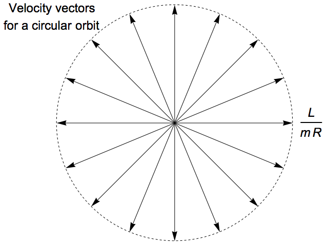
Say the planet has a mass of m and an angular momentum of L. We can find its speed v by solving the equation L = m v R. So the radius of the circle of velocity vectors is v = L / (m R).
Now, suppose the planet is moving in an elliptical orbit, with a perihelion distance (the distance closest to the sun) of R1, and an aphelion distance (the distance farthest from the sun) of R2. Unlike the previous case, the planet’s speed will vary as it moves around the orbit.

As well as knowing R1 and R2, it will be useful to know the major and minor semi-axes of the ellipse, which are traditionally referred to as a and b respectively. These are the largest and smallest distances from the centre of the ellipse to the curve, as opposed to the smallest and largest distances from one focus, R1 and R2.
It’s clear that the semi-major axis a will be given by the arithmetic mean of R1 and R2:
a = ½(R1 + R2)
Less obviously, the semi-minor axis b turns out to be the geometric mean of R1 and R2. The geometric mean of two numbers is defined as the square root of their product:
b = √(R1 R2)
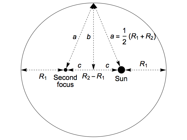
To prove this, we start by noting that by symmetry, the second focus has to be a distance of R1 from the left-most point of the ellipse, which makes the distance between the foci equal to R2 – R1. Traditionally, half of this, the distance from the centre of the ellipse to either focus, is known as c, and we have:
c = ½(R2 – R1)
Next, we use the property of an ellipse that the sum of the distances from the two foci to any point on the curve is constant. For our ellipse, this constant sum is 2 a = R1 + R2. A point equidistant from both foci will lie at a distance of a = ½(R1 + R2), while its distance from the centre of the ellipse is b. Then Pythagoras’s Theorem gives us:
b2 = a2 – c2
= (a – c) (a + c)
= R1 R2
What do the velocity vectors for this elliptical orbit look like, when we gather them all together? The angular momentum of the planet around the sun is equal to the product of its mass, its speed, and the distance between the planet and the sun measured perpendicular to the velocity vector, so we can immediately solve for the velocity at the four locations where the vector is either parallel or perpendicular to the axis of the ellipse:

Surprisingly, these four points lie on a perfect circle! The main difference from the case of a circular orbit is that the centre of the velocity circle is offset from the origin of the vectors:
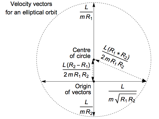
Here, we’ve simply put the centre midway between the top and bottom points, and then the test for circularity is using Pythagoras’s Theorem to check that the distance to the side points is the same as the distance to the top and bottom points. This is easy if we note that:
Distance to the top and bottom points = L (R1 + R2) / (2 m R1 R2) = a L / (m R1 R2)
Horizontal distance to side points = L / (m √(R1 R2)) = b L / (m R1 R2)
Vertical distance to side points = L (R2 – R1) / (2 m R1 R2) = c L / (m R1 R2)
Since a2 = b2 + c2, the same relationship holds for the versions of these quantities multiplied by L / (m R1 R2) that appear in the diagram.
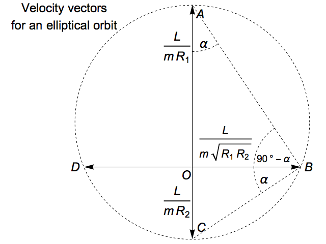
Another way to see this is to make use of the fact that, in the diagram above, the right-angled triangles OAB and OBC have the same ratio of side lengths:
OA/OB = √(R1 R2) / R1 = √(R2 / R1)
OB/OC = R2 / √(R1 R2) = √(R2 / R1)
This makes them similar triangles, with the same angle (say α) as the angle OAB and the angle OBC. It follows that the angle ABC is a right angle. The circle that passes through the three vertices of any right-angled triangle has the hypotenuse as a diameter, and so by symmetry the fourth vector (whose tip is point D here), lies on the same circle.
To prove that all the velocity vectors, not just these four, lie on the same circle, we need to do a little more work. Using coordinates with their origin at the right-most focus of the orbit (that is, the sun), we’ll write an arbitrary point on the orbit as:
r(θ) = r(θ) (cos θ, sin θ)
The other focus will be at (–(R2 – R1), 0). So in order for the sum of the distances from the two foci to be equal to R1 + R2, the distance r(θ) must satisfy the equation:
[R1 + R2 – r(θ)]2 = [r(θ) cos θ + R2 – R1]2 + r(θ)2 sin2 θ
A lot of terms cancel in this equation, and it’s easily solved to give:
r(θ) = 2 R1 R2 / (R1 + R2 + (R2 – R1) cos θ)
To find the velocity of the planet, we take the derivative with respect to time:
v(θ) = dr(θ)/dt = dr(θ)/dθ × dθ/dt
The angular velocity dθ/dt can be found in terms of the angular momentum and the distance from the sun:
dθ/dt = L / (m r(θ)2)
The derivative of the position with respect to θ is, by the product rule:
dr(θ)/dθ = dr(θ)/dθ (cos θ, sin θ) + r(θ) (–sin θ, cos θ)
dr(θ)/dθ = 2 R1 R2 (R2 – R1) sin θ / (R1 + R2 + (R2 – R1) cos θ)2
Putting the pieces together, we end up with:
v(θ) = [L / (2 m R1 R2)] [(0, R2 – R1) + (R1 + R2) (–sin θ, cos θ)]
So the velocities trace out a perfect circle with centre (0, L (R2 – R1) / (2 m R1 R2)) and radius L (R1 + R2) / (2 m R1 R2), which is precisely the circle we’ve already identified as passing through our four original points.
Given a planet orbiting the sun with a certain total energy E – the sum of its kinetic energy, due to its velocity, and its gravitational potential energy, due to its distance from the sun – what other orbits will have the same energy?
We can write the total energy in terms of L, m, R1 and R2. First we find the energy of the planet in terms that include the gravitational constant G and the mass of the sun MS:
E = Kinetic energy at perihelion + Potential energy at perihelion
= ½ m v2Perihelion – G MS m / R1
= ½ L2 / (m R12) – G MS m / R1
Of course we can equally well compute this at aphelion, which gives us:
E = ½ L2 / (m R22) – G MS m / R2
If we equate these two expressions for energy and solve for G MS, we find:
G MS = L2 (R1 + R2) / (2 m2 R1 R2)
If we then substitute that back into either expression for the energy, we get:
E = –L2 / (2 m R1 R2)
If we compute the speed of a planet moving parallel to the axis of its orbit, we see that it depends only on the total energy, E, and the mass of the planet, m:
vParallel = L/(m √(R1 R2)) = √(–2 E/m)
Now, one way to find orbits with the same energy is by applying a rotation that leaves the sun fixed but repositions the planet. Any ordinary three-dimensional rotation can be used in this way, yielding another orbit with exactly the same shape, but oriented differently.
But there is another transformation we can use to give us a new orbit without changing the total energy. If we grab hold of the planet at either of the points where it’s travelling parallel to the axis of the ellipse, and then swing it along a circular arc centred on the sun, we can reposition it without altering its distance from the sun. But rather than rotating its velocity in the same fashion (as we would do if we wanted to rotate the orbit as a whole) we leave its velocity vector unchanged: its direction, as well as its length, stays the same.

Since we haven’t changed the planet’s distance from the sun, its potential energy is unaltered, and since we haven’t changed its velocity, its kinetic energy is the same. What’s more, since the speed of a planet of a given mass when it’s moving parallel to the axis of its orbit depends only on its total energy, the planet will still be in that state with respect to its new orbit, and so the new orbit’s axis must be parallel to the axis of the original orbit.
The orbits we create by this process will (a) all have the same energy, (b) all share a common axis, and (c) all have the same two opposing velocities at the two points when the planet is moving parallel to the orbit’s axis. In terms of the circles traced out by the velocities, this means those circles will all intersect at the two points corresponding to velocities parallel to the axis.

Now, another way to generate exactly the same family of circles is by stereographic projection from a sphere of the appropriate size, sitting tangent to the plane in which the velocity circles lie. We draw lines from the “north pole” of this sphere, through points that lie on a great circle that passes through both ends of a horizontal diameter of the sphere, and continue the lines until they hit the plane. This projects each such great circle onto one of the velocity circles.
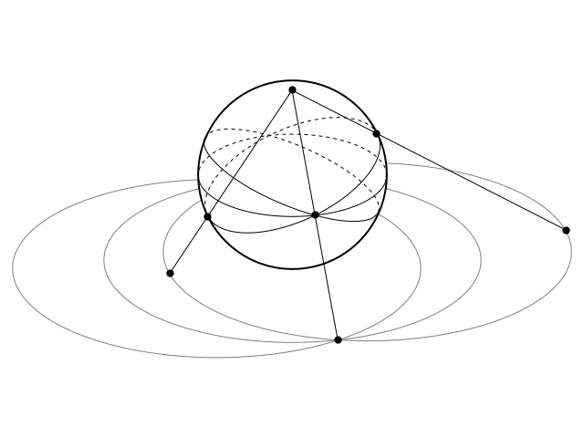
The radius s of this sphere must be half the speed of the planet when it’s moving parallel to the axis of the orbit:
s = ½ √(–2 E/m)
This ensures that the projected distance from the origin when the line from the north pole hits the plane is twice this, giving the point of intersection of all the relevant velocity circles.
We will adopt coordinates where the plane of the velocity circles is z=–s, the centre of the sphere is (0, 0, 0), and the north pole is (0, 0, s). The x-axis will correspond to the axis of our elliptical orbits. An arbitrary point (x, y, z) in the three-dimensional space above the velocity plane is projected onto the plane at:
S(x, y, z) = [2 s / (s – z)] (x, y)
where we omit the constant z-coordinate of –s from the projection and just treat S as mapping into a two-dimensional plane.
The equator of the sphere will simply map into the velocity circle corresponding to a circular orbit, centred on the origin and with a radius of √(–2 E/m). If we tilt the equator around the x-axis by some angle α, a general point on this tilted circle will take the form (s cos θ, s cos α sin θ, s sin α sin θ). The projection of this point is:
S(s cos θ, s cos α sin θ, s sin α sin θ) = [2 s / (1 – sin α sin θ)] (cos θ, cos α sin θ)
The projected points all lie on a circle with centre (0, 2 s tan α) and radius 2 s sec α.
It will be convenient at this point to work with the “force constant” k for the orbit, which includes the gravitational constant, G, the mass of the sun, MS, and the mass of the planet, m:
k = G MS m = L2 (R1 + R2) / (2 m R1 R2)
The radius of the velocity circle, which we found previously to be L (R1 + R2) / (2 m R1 R2), can be expressed in terms of the force constant and the angular momentum:
Radius of circle = k / L
So we have:
2 s sec α = k / L
L √(–2 E/m) = k cos α
The singular case α=π/2, where the velocity circle becomes infinitely large, corresponds to an orbit with zero angular momentum: the planet crashes into the sun, and in this idealised model where the sun is a point mass, the falling planet is accelerated up to infinite velocity.
So far we’ve mostly been treating the planet’s orbit as lying in a fixed plane, but of course the orbit can lie in any plane. So rather than projecting from a sphere in three-dimensional space down to a plane, the more general situation will involve projecting from a 3-sphere (the three-dimensional surface of a four-dimensional ball) down to three dimensions. Any great circle on that 3-sphere will still project onto a velocity circle, but the velocity circles can now be oriented arbitrarily in three-dimensional space. And any four-dimensional rotation applied to a 3-sphere of radius s will take a great circle that corresponds to one orbit of energy E into another great circle corresponding to another orbit with the same energy.
Suppose we rotate a three-dimensional object around the z-axis by some angle θ. The change in the coordinates of any point on the object can be described with the aid of a matrix, which we’ll call Rxy(θ):
| Rxy(θ) | = |
|
We find the new coordinates of a point in the rotated object by matrix multiplication:
r' = Rxy(θ) r
where r=(x, y, z) are the old coordinates and r'=(x', y', z') are the new coordinates. For example, the effect of this rotation on each of the coordinate axes is:
Rxy(θ) (1, 0, 0) = (cos(θ), sin(θ), 0)
Rxy(θ) (0, 1, 0) = (–sin(θ), cos(θ), 0)
Rxy(θ) (0, 0, 1) = (0, 0, 1)
Why do we call the matrix Rxy(θ), rather than Rz(θ), given that it rotates around the z-axis? The z coordinate is unchanged by a rotation around the z-axis, so we’re choosing to describe this rotation in terms of the coordinates that are changed, x and y. This scheme generalises easily to more than three dimensions, where the simplest rotations are those that only affect a given pair of coordinates, while all the remaining coordinates (however many that might be) are left unaltered.
We can construct similar matrices for rotations around the x and y axes, or indeed rotations around any axis at all. And we can find the net effect of two or more successive rotations by multiplying together the relevant matrices. For example, if we rotate an object first by an angle θ around the z-axis and then by an angle φ around the x-axis, the net effect will be to multiply its original coordinates by the matrix:
T = Ryz(φ) Rxy(θ)
The matrix describing the first rotation appears on the right, because we place the original coordinates on the right when calculating the effect of the rotation. Matrix multiplication is not commutative: the order of multiplication matters, so Ryz(φ) Rxy(θ) will not be equal to Rxy(θ) Ryz(φ). And of course this reflects the geometrical reality of rotations: rotating an object around two different axes has a different net effect depending on which rotation you perform first.
It turns out that a very powerful way to get a handle on this non-commutativity is to work, not with rotation matrices, but the matrices we get if we describe a rotation by an angle θ, take the derivative of that matrix with respect to θ, and then set θ equal to 0. For example:
| Jxy | = | dRxy(θ) /dθ |θ=0 | ||||||||||||
| = |
|
|||||||||||||
| = |
|
Physically, what this corresponds to is an angular velocity matrix: the matrix we would use to multiply the coordinates of points on an object in order to obtain their velocity if the object was rotating around a given axis. In that case we would have θ=ωt and we would take the derivative with respect to t, but the only difference that would produce is to multiply the matrix by an overall factor of ω. Similarly, we have:
| Jyz | = | dRyz(θ) /dθ |θ=0 | ||||||||||||
| = |
|
|||||||||||||
| = |
|
|||||||||||||
| Jzx | = | dRzx(θ) /dθ |θ=0 | ||||||||||||
| = |
|
|||||||||||||
| = |
|
|||||||||||||
All three of these matrices are antisymmetric: flipping them around their diagonal so that rows become columns and vice versa negates the whole matrix. The set of all 3 × 3 antisymmetric matrices can be viewed as a three-dimensional vector space, and it turns out that if we rotate around any axis we always get an antisymmetric matrix which can be written as a linear combination of these three. If the axis of rotation is a=(ax, ay, az), the corresponding angular velocity matrix is:
Ja = ax Jyz + ay Jzx + az Jxy
These J matrices don’t commute, but the way in which they fail to do so can be captured more simply than for the rotation matrices. First, we define the commutator for any two matrices as:
[A, B] = A B – B A
Clearly the commutator will be zero if the two matrices commute and A B = B A. For the J matrices for the three coordinate pairs, the commutators turn out to be remarkably simple:
[Jyz, Jzx] = Jxy
[Jzx, Jxy] = Jyz
[Jxy, Jyz] = Jzx
These three equations essentially cover every possibility, because reversing the order of the matrices in the commutator brackets will always just negate the result ([B, A] = –[A, B]), and if the same matrix appears twice then it commutes with itself ([A, A] = 0).
Now, to make a connection with quantum mechanics, consider the operators on functions of three coordinates, say f(x, y, z), defined by:
Lxy f = –iℏ (x ∂y f – y ∂x f)
Lyz f = –iℏ (y ∂z f – z ∂y f)
Lzx f = –iℏ (z ∂x f – x ∂z f)
where i is the square root of minus one and ℏ is the “reduced Planck’s constant”, ℏ=h/(2π). We can calculate the commutators of these L operators, where instead of matrix multiplication we just apply the operators in succession to a function f(x, y, z), i.e.
[Lyz, Lzx] f = Lyz(Lzx f ) – Lzx(Lyz f )
Making use of the definitions we get:
[Lyz, Lzx] = iℏ Lxy
[Lzx, Lxy] = iℏ Lyz
[Lxy, Lyz] = iℏ Lzx
Clearly the pattern here mimics the commutators of the J matrices very closely. We can talk about this mimicry more formally by saying that we have a representation of the algebra of three-dimensional rotations (the vector space of J matrices, which is known as so(3)) on the vector space of functions of three-dimensional space, given by associating each J matrix with the corresponding L operator. If we define:
dρ(Jαβ)=Lαβ/(iℏ)
(where αβ stands for any pair of coordinates), we can extend dρ to any linear combination of the coordinate J matrices by requiring that dρ be a linear function. We then have:
[dρ(Ja), dρ(Jb)] = dρ([Ja, Jb])
So what we mean by a representation is a function like dρ that “preserves” the commutator in this sense: we can take the commutator of the original matrices and then apply the function, or we can apply the function first and then take the commutator, and it makes no difference to the result.
What are these L operators? In quantum mechanics, we obtain the component of a particle’s momentum in a given direction by taking the derivative of the particle’s wave function ψ(x, y, z) in that direction, and multiplying by –iℏ. For example, the momentum in the x direction is given by:
px ψ(x, y, z) = –iℏ ∂x ψ(x, y, z)
When the wave function describes a particle with a definite value for some quantity like momentum, the corresponding operator simply multiplies the wave function by that value. So, for example, if the wave function were given by ψ(x, y, z)=exp(i P x / ℏ), we would have:
px ψ(x, y, z) = –iℏ ∂x exp(i P x / ℏ) = P exp(i P x / ℏ) = P ψ(x, y, z)
So that particular wave function has a definite value of P for the x component of its momentum, and we say that it is an eigenfunction of the momentum operator, with eigenvalue P.
The angular momentum vector, L, of a classical particle is given by the vector cross product of the particle’s position and momentum vectors:
L = r × p
If we expand out the cross product for the individual coordinates, and then convert the momentum coordinates to their quantum-mechanical equivalents, we get:
Lx = y pz – z py → –iℏ (y ∂z – z ∂y) = Lyz
Ly = z px – x pz → –iℏ (z ∂x – x ∂z) = Lzx
Lz = x py – y px → –iℏ (x ∂y – y ∂x) = Lxy
So these L operators are the quantum-mechanical equivalents of the coordinates of the particle’s angular momentum vector. The similarity between their commutators and those of the J matrices isn’t too surprising, given that the J matrices are essentially tools for computing angular velocities, and for a single particle its angular momentum is just its mass times its angular velocity.
We can construct an operator that corresponds to the squared magnitude of the angular momentum vector:
L2 f = Lyz(Lyz f ) + Lzx(Lzx f ) + Lxy(Lxy f )
This operator, L2, commutes with all the individual components of the angular momentum.
Now, we’d like to identify various vector spaces of wave functions that are invariant under rotation: that is, if ψ(r) is a function in the vector space, and R is a rotation, then ψR(r) = ψ(R r) is also in the same vector space. [Note that it’s the vector space as a whole that is invariant. We’re not saying that the individual functions in the space are unchanged by rotations.] Physically, if we rotate a self-contained quantum system (or describe the same system in a new, rotated set of coordinates), its wave function will change, and we would like to know what kinds of vector spaces of functions contain all the wave functions we can get by performing such a rotation on any given function in the space.
One example of a space of functions that will be invariant under rotations is the set of all homogeneous polynomials of a given degree in x, y and z. A homogeneous polynomial is one where the sum of the powers of all its variables is the same in every term. That sum is called the degree of the polynomial. For example:
f(x, y, z) = 7 x2 y z + 3 x y z2
is a homogeneous polynomial of degree four. It’s not hard to see that if we perform any linear transformation of our coordinates – that is, we replace each coordinate by some linear combination of the three original coordinates — we will still have a homogeneous polynomial of the same degree. Since a rotation is a linear transformation, the space of homogeneous polynomials of any particular degree will be invariant under rotations.
To make things even simpler, we would like to find a space of functions that, as well as being invariant under rotations, can’t be broken down into any smaller spaces that are themselves invariant. We’ll call such a space irreducible. It turns out that the space of homogeneous polynomials of a given degree does contain a smaller invariant space: those polynomials that are also solutions of Laplace’s equation:
∇2 f = 0
where in three-dimensions we define the Laplacian operator ∇2 as the sum of the second derivatives with respect to the three coordinates:
∇2 f = ∂x, x f + ∂y, y f + ∂z, z f
To see why the property of satisfying Laplace’s equation is unchanged under a rotation, just change to a new Cartesian coordinate system related to the first by a rotation. If we write the three original coordinates as xj for j=1,2,3, we can write the Laplacian operator as:
∇2 f = Σj ∂xj, xj f
Our new, rotated coordinates ξi will be related to the old coordinates by:
ξi = Σj Rij xj
where Rij are the coordinates of the rotation matrix. We then have, making use of the chain rule for derivatives:
∇2 f = Σj ∂xj, xj f
= Σj Σα Σβ (∂xj ξα) (∂xj ξβ) ∂ξα, ξβ f
= Σj Σα Σβ Rα j Rβ j ∂ξα, ξβ f
= Σα Σβ (Σj Rα j Rβ j) ∂ξα, ξβ f
= Σα Σβ δαβ ∂ξα, ξβ f
= Σα ∂ξα, ξα f
which is just the Laplacian in the new coordinates. In the step:
Σj Rα j Rβ j = δαβ
the symbol δαβ is known as the Kronecker delta, which is equal to 1 when α and β are equal and 0 otherwise. This step amounts to claiming that the product of the rotation matrix and its transpose is the identity matrix, or, equivalently, that the dot product of any two rows of the matrix will be 0 if they are different rows and 1 if they are the same. It’s easy to see that this must be true for the columns of the rotation matrix, since the columns are the vectors produced by rotating each of the coordinate axes. The statement about the columns corresponds to the matrix equation RTR=I, while the statement about the rows corresponds to RRT=I. But every invertible matrix only has a single inverse, and it makes no difference whether we multiply by the inverse on the left or the right. So RT is the inverse of R, and the statement about the rows is also true.
A solid spherical harmonic is a homogeneous polynomial in the Cartesian coordinates that satisfies Laplace’s equation. We will refer to a solid spherical harmonic of degree λ as Zλ, σ(x, y, z), where λ is an integer greater than or equal to zero, and the second subscript σ stands for some as-yet-unspecified way of labelling individual polynomials. For any fixed value of λ, the space spanned by these functions is invariant under rotations, and also irreducible: it contains no smaller invariant space.
We will define the ordinary (as opposed to the solid) spherical harmonic for unit vectors u as:
Yλ, σ(u) = Zλ, σ(u)
So Yλ, σ is defined only on the unit sphere S2, where it agrees with Zλ, σ. Because the solid spherical harmonics are homogeneous polynomials, they scale with the power of λ, giving us:
Zλ, σ(r) = rλ Zλ, σ(r/r) = rλ Yλ, σ(r/r)
If we apply the operator L2 to Zλ, σ, and make use of the fact that Zλ, σ is a solution of Laplace’s equation, we obtain the result:
L2 Zλ, σ(r) = ℏ2 λ(λ+1) Zλ, σ(r) – ℏ2 r2 ∇2 Zλ, σ(r)
= ℏ2 λ(λ+1) Zλ, σ(r)
So all the solid spherical harmonics of degree λ are eigenfunctions of the squared angular momentum operator, with eigenvalue ℏ2 λ(λ+1). The same will be true for any linear combination of the Zλ, σ with the same λ. So for each invariant space of functions like this we have a distinct value for the squared angular momentum.
We will refer to the space of functions spanned by the Zλ, σ as the spin-λ representation of the rotation algebra. To find its dimension, first we note that with two variables, it’s easy to see that the number of possible monomials of degree λ is just λ+1, since we can give the first variable any power from 0 to λ and then we have no choice for the second variable. With three variables, we can take any two-variable monomial of degree ranging from 0 up to λ and multiply it by the third variable raised to an appropriate power, so we have a total of:
1 + 2 + ... + (λ+1) = ½(λ+2)(λ+1)
The Laplacian operator reduces the degree of a homogeneous polynomial by two, so requiring it to be zero imposes ½λ(λ–1) constraints. That leaves the dimension of the space equal to the difference of these two expressions, which is 2λ+1. So the spin-λ representation has dimension 2λ+1.
To interpret this more physically, we can choose a basis of the space in which each element of the basis has a different eigenvalue for one of the L operators: for example, Lxy, which measures the z component of the angular momentum vector. If we define:
Zλ, λ(x, y, z) = (x + i y)λ
then this is clearly a homogeneous polynomial of degree λ, and it’s a straightforward calculation to show that:
∇2 Zλ, λ = 0
Lxy Zλ, λ = λℏ Zλ, λ
So we’ve identified one function in the spin-λ representation which has a z component of its angular momentum of exactly λ (measured in the quantum units of spin, ℏ). Similarly, we can define a function whose z component of angular momentum is the opposite of this:
Zλ, –λ(x, y, z) = (x – i y)λ
∇2 Zλ, –λ = 0
Lxy Zλ, –λ = –λℏ Zλ, –λ
Now, suppose we’re given a function Zλ, m which is an eigenfunction of Lxy with eigenvalue mℏ. In what follows, we will make use of the commutators between the L operators:
[Lxy, Lyz] = iℏ Lzx
Lxy Lyz = iℏ Lzx + Lyz Lxy
[Lzx, Lxy] = iℏ Lyz
–Lxy Lzx = iℏ Lyz – Lzx Lxy
We now define a “spin-lowering operator”:
L– = Lyz – i Lzx
If we apply this operator to Zλ, m, an existing eigenfunction of Lxy with eigenvalue mℏ, we get:
Lxy (L– Zλ, m)
= Lxy (Lyz – i Lzx) Zλ, m
= (Lxy Lyz – i Lxy Lzx) Zλ, m
= (iℏ Lzx + Lyz Lxy + i (iℏ Lyz – Lzx Lxy)) Zλ, m
= (iℏ Lzx + mℏ Lyz + i (iℏ Lyz – mℏ Lzx)) Zλ, m
= (m–1) ℏ (Lyz – i Lzx) Zλ, m
= (m–1) ℏ (L– Zλ, m)
So L– gives us a new eigenfunction of Lxy with an eigenvalue that is one unit less than that of the function we started with. However, this process can’t go on forever. If we apply the spin-lowering operator to Zλ, –λ, we get:
L– Zλ, –λ
= (Lyz – i Lzx) (x – i y)λ
= –iℏ (y ∂z – z ∂y – i z ∂x + i x ∂z) (x – i y)λ
= iℏ z (∂y + i ∂x) (x – i y)λ
= 0
So we get a basis {Zλ, –λ, Zλ, –λ+1, ..., Zλ, λ–1, Zλ, λ} of the spin-λ representation, with exactly 2λ+1 elements, each of which is an eigenfunction of Lxy with an eigenvalue that varies in integer units from –λ up to λ.
Though we won’t prove it, it turns out that all irreducible representations of the rotation algebra have an identical structure to the function spaces that we’ve called the spin-λ representations: they can all be characterised by a number λ related to their dimension 2λ+1, and they can all be given a basis of eigenvectors of one of the angular momentum components, with eigenvalues that range (in suitable units) from –λ to λ in integer steps. The only aspect that can’t be seen in our examples of spaces of wave functions is that it’s possible to have a representation where λ takes, not an integer value, but a half-integer value. For example, the vector space for the intrinsic spin of an electron is the spin-½ representation, a two-dimensional vector space, and the z component of an electron’s spin can have eigenvalues of either –½ℏ or ½ℏ.
If we extend the ideas from the previous section to a space with four dimensions (adding a coordinate w alongside the original x, y and z), then we can define rotation matrices in a similar way to encompass the three new pairs of coordinates, and take their derivatives to obtain three new J matrices: Jxw, Jyw, Jzw. The four-dimensional rotation algebra can be summed up by saying that when i, j and k are distinct:
[Jij, Jkj] = Jik
Apart from rearrangements of this basic identity with appropriate changes of sign, all other commutators are zero. That’s simple enough, but it turns out that there’s a different choice of matrices that makes things even simpler.
|
|
|
||||||||||||||||||||||||||||||||||||||||||||||||||||||||||||||||||
|
|
|
For these matrices, the commutators are:
[Ax, Ay] = Az, and cyclic permutations
[Bx, By] = Bz, and cyclic permutations
[Ai, Bj] = 0, for all i and j.
So there are individual “sub-algebras” formed by the A and B matrices that have exactly the same structure as the three-dimensional rotation algebra so(3), and all the commutators between the two sub-algebras are zero.
In general, then, we’d expect to describe an irreducible representation of the four-dimensional rotation algebra, so(4), by choosing two numbers, λA and λB, and combining the spin-λA and the spin-λB representations of the three-dimensional rotation algebra, so(3). Since we can define spin-lowering operators that act indepently on the Az or Bz eigenvalues, those eigenvalues will vary independently across their respective ranges, and we will have a total of (2λA+1)(2λB+1) different vectors as a basis for the whole space.
However, if we work with functions on four-dimensional space and extend the L operators to all six pairs of coordinates, for these representations we will always have λA=λB. The reason for this is that these functions describe the quantum mechanics of a single particle, and while a completely general angular velocity in four dimensions can involve an arbitrary linear combination of the six J matrices, the angular velocity of a point particle always entails motion in a single plane: the plane spanned by the vector giving the particle’s position relative to the origin, and the vector for its velocity.
Suppose we rewrite the angular velocity as a linear combination of the A and B matrices:
J = ax Ax + ay Ay + az Az + bx Bx + by By + bz Bz
Since the motion lies in a single plane, we could always choose coordinates such that:
J = ω Jxy = ω Az + ω Bz
ax = ay = bx = by = 0
az = bz = ω
ax2 + ay2 + az2 = bx2 + by2 + bz2
The exact values of ax, bx etc. depend on the choice of coordinates, but the last line, where the sum of the squares of both triples of coefficients are the same, can be shown to be independent of the coordinate system. So for any simple rotation (a rotation in a single plane), the triples of coefficients for the A and B matrices have the same squared magnitude.
To prove the quantum-mechanical version of this result, the notation will be simpler if we define some three-dimensional vectors of operators:
L = (Lyz, Lzx, Lxy)
M = (Lxw, Lyw, Lzw)
A = ½(L + M)
B = ½(L – M)
Here we’re using the same letters, A and B, for the sums and differences we form from the L operators as we used for the matrices formed from the sums and differences of the J matrices. We can define squared angular momentum operators for the two spins:
A2 = A · A = ¼(L · L + L · M + M · L + M · M)
B2 = B · B = ¼(L · L – L · M – M · L + M · M)
A2 – B2 = ½(L · M + M · L)
A2 + B2 = ½(L2 + M2)
Now, if we make use of the definitions of the L operators, we find that:
(L · M) f
= –ℏ2 [ (y ∂z – z ∂y) (x ∂w – w ∂x) + (z ∂x – x ∂z) (y ∂w – w ∂y) + (x ∂y – y ∂x) (z ∂w – w ∂z) ] f
= –ℏ2 [ (x y ∂z, w + z w ∂x, y – x z ∂y, w – y w ∂x, z)
+ (y z ∂x, w + x w ∂y, z – x y ∂z, w – z w ∂x, y)
+ (x z ∂y, w + y w ∂x, z – y z ∂x, w – x w ∂y, z) ] f
= 0
Similarly, (M · L) f = 0. So A2 = B2, and λA=λB.
We define solid spherical harmonics in four dimensions as homogeneous polynomials in the four Cartesian coordinates x, y, z and w that satisfy the four-dimensional version of Laplace’s equation. We will refer to a four-dimensional solid spherical harmonic of degree λ as Zλ, σ, μ, and the ordinary spherical harmonic that agrees with it on the unit sphere as Yλ, σ, μ. There are many different ways we could choose individual functions, but one obvious scheme would be to have σ and μ equal to the eigenvalues of Az and Bz respectively, with both ranging from –λA to λA.
In three dimensions, the squared magnitude of the angular momentum vector, L2, is unchanged by any rotation, and the set of eigenfunctions of L2 with a given eigenvalue form an invariant space. In four dimensions, the angular velocity matrices have six independent components, and any quantity that is left unchanged by rotations needs to include all six, since in general a rotation might shift any one of those components into any other. In the notation we’re using, A2 + B2 and L2 + M2 (which are the same thing except for a factor of ½) are invariant under all rotations, and the four-dimensional solid spherical harmonics are eigenfunctions of both:
(A2 + B2) Zλ, σ, μ(r)
= ½ (L2 + M2) Zλ, σ, μ(r)
= ½ [ℏ2 λ(λ+2) Zλ, σ, μ(r) – ℏ2 r2 ∇2 Zλ, σ, μ(r)]
= ½ℏ2 λ(λ+2) Zλ, σ, μ(r)
The third line above depends only on the function Zλ, σ, μ(r) being homogeneous with degree λ, with the fourth line following because Zλ, σ, μ(r) is also harmonic. Since A2 = B2, this becomes:
A2 Zλ, σ, μ(r)
= ¼ℏ2 λ(λ+2) Zλ, σ, μ(r)
= ℏ2 (½λ)(½λ+1) Zλ, σ, μ(r)
In the spin-λA representation of the three-dimensional rotation algebra, A2 = ℏ2 λA(λA+1), so we must have λA = λB = ½λ. The dimension of the representation we get from the solid spherical harmonics of degree λ is:
(2λA+1)(2λB+1) = (λ+1)2
As a check, we can get the same dimension by directly counting the number of independent polynomials. By a similar argument to that we gave for the three-dimensional spherical harmonics, we can show that there are (λ+3)(λ+2)(λ+1)/6 linearly independent homogeneous polynomials in four variables with degree λ. Then, since the Laplacian operator reduces the degree of a homogeneous polynomial by two, requiring it to be zero imposes (λ+1) λ (λ–1)/6 constraints. That leaves the dimension of the space equal to the difference of these two expressions, which is just (λ+1)2.
To give concrete examples of four-dimensional spherical harmonics, we can start by defining:
Zλ, ½λ, ½λ(x, y, z, w) = (x + i y)λ
This has eigenvalues for both Az and Bz of ½ℏλ. We can then obtain other eigenfunctions with lower spins using the lowering operators:
A– = Ax – i Ay
B– = Bx – i By
Pauli[1][2] found the energy levels of hydrogen by realising that the quantum mechanical equivalent of a suitably-scaled version of a classical vector known as the Laplace-Runge-Lenz vector (which points along the axis of a planet’s elliptical orbit), acts exactly like our vector M, so that the algebra formed by the Laplace-Runge-Lenz vector and the angular momentum vector L was none other than the four-dimensional rotation algebra in disguise! Pauli wasn’t working with functions on four-dimensional space, and he obtained the equation L · M = 0 from the classical relationship between the angular momentum (which is perpendicular to the plane of the orbit) and the Laplace-Runge-Lenz vector, which lies in the plane.
We won’t go into the details of Pauli’s calculations, but there is one aspect of the connection that’s very easy to see. For every ellipse, we have the relationship between the semi-major axis, a, the semi-minor axis, b, and the distance from the centre to each focus, c:
b2 + c2 = a2
For an orbit, fixing the total energy E is enough to fix the semi-major axis, a. The semi-minor axis, b, is then proportional to the angular momentum, L. The length of the Laplace-Runge-Lenz vector, M, is proportional to the eccentricity of the orbit, which in turn is proportional to c. So, given the right choice of an overall factor for M, the invariance of:
L2 + M2
for all orbits with a fixed total energy just reflects the Pythagorean relationship between a, b and c.
To take this a little further, suppose we choose two vectors A and B in three-dimensional space, with the only restriction being:
A2 = B2 = –k2 m/(8 E)
for some fixed total energy E. Clearly we’re free to rotate either vector, independently of the other, without changing this condition. Then if we set:
L = A + B
M = A – B
we have:
L · M = (A + B) · (A – B) = A · A – B · B = 0
L2 + M2 = (A + B) · (A + B) + (A – B) · (A – B) = 2(A2 + B2) = –k2 m/(2 E)
Since L and M are guaranteed to be orthogonal, we can always choose an elliptical orbit whose plane is perpendicular to L and has M pointing in the direction from the centre of attraction to the second focus of the ellipse.
The exact relationships between energy, angular momentum and the semi-major and semi-minor axes of the orbit can be found from two of our earlier results:
E = –L2 / (2 m R1 R2)
k = G MS m = L2 (R1 + R2) / (2 m R1 R2)
a = ½(R1 + R2) = –k/(2 E)
b2 = R1 R2 = –L2/(2 E m)
If we scale M so it’s related to c by the same factor as L and b, we have:
c2 = –M2/(2 E m)
b2 + c2 = –(L2 + M2)/(2 E m) = k2/(4 E2) = a2
So, once we fix E we see that the set of orbits that share the same total energy is invariant under two completely independent rotations of the two vectors A and B, giving the same kind of doubling of the rotation algebra that we see in four-dimensional rotations.
If we set aside the physical vectors and just concentrate on the geometry, there’s an even simpler construction that demonstrates the same symmetries. Choose two vectors A and B whose lengths are equal. Place one focus of an ellipse at the origin, place the second focus at A + B, and position the two points of the ellipse where the tangent to the curve is parallel to its axis at A and B. This construction will always yield an ellipse with a semi-major axis equal to |A| (with the degenerate case of a line when A = B), and the entire family of ellipses with one focus at the origin and the same length for the semi-major axis can be generated by rotating A and B independently.

Of course our B here is more like the opposite of the B used in the previous construction, and the vector A – B whose length is now proportional to the angular momentum lies in the plane of the orbit, not perpendicular to it. But everything can be mapped between the different schemes in a way that preserves the essential feature: the two independent three-dimensional rotations.
In 1935, Vladimir Fock[3] used the stereographic projection from a 3-sphere to momentum space (which is the same as the velocity space we’ve been working with, apart from a factor of m) to analyse the quantum-mechanical solutions for a particle moving under an inverse-square force. Of course in the quantum mechanical case, rather than a star and a planet we’re studying a proton and an electron. I haven’t read Fock’s original paper, so for parts of what follows I’m indebted to the accounts of Jonas Karlsson[4], Radosław Szmytkowski[5] and Bander and Itzykson[6].
The ordinary Schrödinger equation for a particle moving under an inverse-square force with a force constant of k is:
–ℏ2/(2m) ∇2 φ(r) – (k/|r|) φ(r) = E φ(r)
This is the time-independent equation, for an eigenfunction φ(r) with energy E. Here we’ve expressed the particle’s state φ(r) as a function of its position, r. But if we wish, we can express the particle’s state as a function ψ(p) of its momentum, p, instead. The two representations are related by what are essentially Fourier transforms:
φ(r) = 1/√(8 π3 ℏ3) ∫R3 ψ(p) exp(i p·r/ℏ) d3p
ψ(p) = 1/√(8 π3 ℏ3) ∫R3 φ(r) exp(–i p·r/ℏ) d3r
We obtain the momentum-space Schrödinger equation by performing a Fourier transform of the original. The hardest part here is Fourier-transforming the potential energy, –k/|r|. We start by establishing a handy integral representation of 1/r:
∫0∞ [exp(–αr2)/√α] dα
Putting α=β/r2
= 1/r ∫0∞ [exp(–β)/√β] dβ
= Γ(½)/r [where Γ is the Gamma function]
= √(π)/r
So we can write:
1/r = [1/√π] ∫0∞ [exp(–αr2)/√α] dα
In what follows we’ll write the magnitude of any vector using the same letter as we use for the vector itself, but dropping the bold-face, e.g. p for |p| and r for |r|. Using the integral representation of 1/r, the Fourier transform of the potential is:
V(p) = 1/√(8 π3 ℏ3) ∫R3 [–k/r] exp(–i p·r/ℏ) d3r
= –k/√(8 π4 ℏ3) ∫0∞ [1/ √α] ∫R3 exp(–i p·r/ℏ) exp(–αr2) d3r dα
We can transform the integral over R3 into spherical polar coordinates, choosing to measure the angle θ from the direction of the momentum vector p, so that p·r = p r cos θ.
∫R3 exp(–i p·r/ℏ) exp(–αr2) d3r
= ∫02π ∫0∞ ∫0π exp(–i p r cos θ/ℏ) sin θ dθ exp(–αr2) r2 dr dφ
= 2π ∫0∞ ∫0π exp(–i p r cos θ/ℏ) sin θ dθ exp(–αr2) r2 dr
Putting z=cos θ
= 2π ∫0∞ ∫–11 exp(–i p r z/ℏ) dz exp(–αr2) r2 dr
= [2π ℏ i / p] ∫0∞ [ exp(–i p r/ℏ) – exp(i p r/ℏ) ] exp(–αr2) r dr
= [π ℏ i / p] ∫–∞∞ [ exp(–i p r/ℏ) – exp(i p r/ℏ) ] exp(–αr2) r dr
Putting r=u/√α – i p / (2 ℏ α) in the first term, r=u/√α + i p / (2 ℏ α) in the second term
= [π / (2 p α3/2)] exp(–p2 / (4 ℏ2 α))
× [∫–∞∞ exp(–u2) (p + 2 i ℏ u √α) du + ∫–∞∞ exp(–u2) (p – 2 i ℏ u √α) du]
= [π / α3/2] exp(–p2 / (4 ℏ2 α)) ∫–∞∞ exp(–u2) du
= (π/α)3/2 exp(–p2 / (4 ℏ2 α))
We then have:
V(p) = –k/√(8 π ℏ3) ∫0∞ [1/ α2] exp(–p2 / (4 ℏ2 α)) dα
Putting α=p2/(4 ℏ2 γ)
= –k √(2ℏ/π) [1/p2] ∫0∞ exp(–γ) dγ
= –k √(2ℏ/π) [1/p2]
So the Fourier transform of an inverse potential in distance is just an inverse square in the magnitude of the momentum. The Fourier transform of the product of the potential and the original wave function is the convolution of the individual Fourier transforms, so we end up with the momentum-space Schrödinger equation:
[p2/(2m) – E] ψ(p) – [k/(2 π2 ℏ)] ∫R3 [ψ(p')/|p–p'|2] d3p' = 0
[Note that we’ve had to insert a further factor of 1/√(8 π3 ℏ3) into the convolution between the Fourier transforms of the potential and that of the wave function, because of our choice of normalisation in the original Fourier transforms. Different choices there give different results along the way, but the final equation in momentum space will always end up the same.]
Fock’s extraordinary insight was that this integral equation is equivalent to the four-dimensional Laplace equation restricted to the surface of a 3-sphere that we stereographically project onto the three-dimensional momentum space!
The stereographic projection from a 3-sphere of radius s is given by:
S4(x, y, z, w) = [2 s / (s – w)] (x, y, z)
We’re projecting onto a three-dimensional hyperplane tangent to the 3-sphere’s “south pole” at (0,0,0,–s). Note that our s is not the same as when we were projecting onto the velocity circles, because we’re dealing with momentum space with an extra factor of m. For the moment, though, we’ll just leave s as a free parameter.
Starting from the integral over R3 in the momentum-space version of the Schrödinger equation, we want to perform a change of variables to coordinates on the 3-sphere. We will put coordinates on the 3-sphere of η, θ and φ, with:
0 ≤ η ≤ π
0 ≤ θ ≤ π
0 ≤ φ ≤ 2π
Cartesian coordinates are s (sin η sin θ cos φ, sin η sin θ sin φ, sin η cos θ, cos η)
3-volume element is dΩ = s3 sin2 η sin θ dη dθ dφ
Total 3-volume of 3-sphere is 2 π2 s3
If we consider the projection from the generic point s=s (sin η sin θ cos φ, sin η sin θ sin φ, sin η cos θ, cos η), we have:
S4(s) = [2s sin η / (1 – cos η)] (cos φ sin θ, sin φ sin θ, cos θ)
The two angular spherical coordinates in R3, θ and φ, are exactly the same as the corresponding coordinates on the 3-sphere, while the radial coordinate in R3 (which we’ll call p, since we’re in momentum space) and the angular coordinate η are related by:
p = 2s sin η / (1 – cos η)
We’ll shortly need the derivative of this, which turns out to be:
dp/dη = –2s / (1 – cos η)
If we change from p to η, the volume element on momentum space becomes:
Momentum-space 3-volume element
d3p = p2 sin θ dp dθ dφ
= 4s2 sin2 η / (1 – cos η)2 |dp/dη| sin θ dη dθ dφ
= 8s3 sin2 η / (1 – cos η)3 sin θ dη dθ dφ
= 8 / (1 – cos η)3 dΩ
We can re-express the function of η here by noting that:
p2 + 4 s2 = 4 s2 (1 + sin2 η / (1 – cos η)2)
= 4 s2 (1 – 2 cos η + cos2 η + sin2 η) / (1 – cos η)2
= 8 s2 (1 – cos η) / (1 – cos η)2
= 8 s2 / (1 – cos η)
So we have:
d3p = (p2/(4 s2) + 1)3 dΩ
The inverse projection from a point (X, Y, Z) in the three-dimensional hyperplane to a point on the 3-sphere is:
R4(X, Y, Z) = (4 s2 X, 4 s2 Y, 4 s2 Z, s (X 2 + Y 2 + Z 2 – 4 s2)) / (X 2 + Y 2 + Z 2+ 4 s2)
From this, we find:
|p–p'|2 = [p2/(4 s2) + 1][p'2/(4 s2) + 1] |R4(p) – R4(p')|2
If we write s=R4(p) and s'=R4(p'), and define:
Ψ(s) = [p2/(4 s2) + 1]2 ψ(p)
then our original integral over R3 becomes:
∫R3 [ψ(p')/|p–p'|2] d3p' = 1/[p2/(4 s2) + 1] ∫s S3 [Ψ(s')/|s–s'|2] dΩ'
Here we’re writing the surface of the ball of radius s as s S3, where S3 is taken to be the unit-radius 3-sphere in R4. We set the value of s to √(–½ E m), which is just m times the value we used for velocity space. This means that:
–E = 2 s2 / m
p2/(2 m) – E = (2 s2 / m) × (p2/(4 s2) + 1)
and the momentum-space Schrödinger equation becomes:
Ψ(s) – [m/(2 s2)][k/(2 π2 ℏ)] ∫s S3 [Ψ(s')/|s–s'|2] dΩ' = 0
This equation is invariant under any four-dimensional rotation: if Ψ(s) is a solution, and R is a rotation of R4, then ΨR(s)=Ψ(R s) will solve the equation too. To prove this, all we have to do is change the variable of integration from s' to s''=R s', which has no effect on the volume element or the set over which we’re integrating, and which gives us |s–s'|=|R s–R s'|=|R s–s''|.
Now consider the function:
P(r, s) = 1 / |r – s|2 = 1 / [(r – s) · (r – s)]
where r and s are vectors in R4. We claim that P(r, s) is a solution of the four-dimensional Laplace equation, if we hold s fixed and treat P(r, s) as a function of the four-dimensional vector r alone. To see this, we first look at the derivatives with respect to an individual coordinate, say x, where r=(x, y, z, w) and s=(sx, sy, sz, sw).
∂xP(r, s) = –2 (x – sx) / [(r – s) · (r – s)]2
∂x, xP(r, s) = –2 / [(r – s) · (r – s)]2 + 8 (x – sx)2 / [(r – s) · (r – s)]3
Adding up the equivalent terms for all four coordinates, we get:
∇2P(r, s) = –8 / [(r – s) · (r – s)]2 + 8 [(r – s) · (r – s)] / [(r – s) · (r – s)]3 = 0
This calculation goes through nicely when r ≠ s, but of course P(r, s) is singular when r = s. In fact, rather than ∇2P(r, s)=0, we have:
∇2P(r, s) = –4 π2 δ(r – s)
where δ is the Dirac delta function, a generalised function or distribution with the property that integrating the product of any “test function” f(r) and the Dirac delta δ(r – s) gives the value of f at r=s. We won’t give a rigorous proof of this, but to make this claim plausible we note first that the gradient of P(r, s) is given by:
∇P(r, s) = –2 (r – s) / [(r – s) · (r – s)]2
We can find the integral of the Laplacian throughout a unit solid ball in R4 centred on s (which we’ll describe as s+B4, with B4 the unit sold ball centred on the origin) by noting that the Laplacian is just the divergence of the gradient, and applying the divergence theorem to compute this as an integral over the ball’s three-dimensional boundary. That boundary is a unit 3-sphere, s+S3, and the unit outwards normal at any point r on it is just r – s. So we have:
∫s+B4 ∇2P(r, s) d4r
= ∫s+B4 ∇ · ∇P(r, s) d4r
= ∫s+S3 (r – s) · ∇P(r, s) dΩ
= –2 ∫s+S3 dΩ
= –4 π2
Given that P(r, s) is a solution of Laplace’s equation, at least for r ≠ s, and that Ψ(s) in our equation on the 3-sphere is an integral over s' of P(s, s'), it seems plausible that Ψ(s) itself should satisfy Laplace’s equation. To make progress in seeing exactly which solutions will work, we will substitute a four-dimensional spherical harmonic:
Ψ(s) = Zλ, σ, μ(s)
into our transformed Schrödinger equation on the 3-sphere s S3. In order to evaluate the integral ∫s S3 [Zλ, σ, μ(s')/|s–s'|2] dΩ' we will make use of a form of Green’s second identity, which is a result that follows easily from the divergence theorem:
∫V (f ∇2 g – g ∇2 f) d4r = ∫Boundary of V n · (f ∇g – g ∇f) dΩ
Here n is a unit outwards normal to the four-dimensional set V over which we’re integrating on the left-hand side. To apply this identity we will set f = Zλ, σ, μ and g=P(s', s)=1/|s–s'|2. Rather than integrating over the entire four-dimensional ball s B4, we will exclude a piece of radius ε that contains the point s, and then let ε go to zero. That is, we will define the set over which we integrate as:
V = {s' in R4 such that |s'| ≤ s and |s–s'| ≥ ε}
This has the advantage that both f and g are solutions of Laplace’s equation on V, so the left-hand side of Green’s identity, the integral over V of an expression that contains the Laplacians, is simply zero. So we end up with:
∫Boundary of V Zλ, σ, μ(s') (n · ∇P(s', s)) dΩ' = ∫Boundary of V P(s', s) (n · ∇Zλ, σ, μ(s')) dΩ'
The boundary of V will consist of two pieces. One piece is the 3-sphere s S3 excluding those points closer to s than ε. The other piece will approximate a half-3-sphere centred on s, of radius ε.
On the 3-sphere s S3, the dot product of the outwards normal, n, with the gradient of the solid spherical harmonic is just the rate of change of the solid spherical harmonic with distance from the origin. From the homogeneity of the polynomial, this evaluates to a multiple of the original function:
n · ∇Zλ, σ, μ(s')
= ∂r Zλ, σ, μ(r (s' / s))|r=s
= ∂r [rλ Yλ, σ, μ(s' / s)]|r=s
= λ rλ–1 Yλ, σ, μ(s' / s)|r=s
= [λ / s] Zλ, σ, μ(s')
And again on the 3-sphere s S3, the dot product of the outwards normal, n, with the gradient of P(s', s) turns out to be a multiple of the original function:
∇P(r, s) = –2 (r – s) / [(r – s) · (r – s)]2
(r / r) · ∇P(r, s)|r=s
= –[2/s] (s – r · s) / (2 s – 2 r · s)2
= –1 / [2 s (s – r · s)]
P(r, s)|r=s
= 1 / [(r – s) · (r – s)]|r=s
= 1 / [2 (s – r · s)]
Putting r=s', we have on the 3-sphere s S3:
n · ∇P(s', s) = [–1/s] P(s', s)
The other piece of the boundary of V is the (approximate) half-3-sphere around the point s, with radius ε. The integral on any complete 3-sphere around s of the dot product of the outwards normal with the gradient ∇P(s', s) will just be –4 π2, as we found previously when showing that the Laplacian of P is a multiple of the Dirac delta. Because P(s', s) is radially symmetrical about s, as ε tends to zero one of the integrals over this part of the boundary of V will approach:
∫Half-3-sphere around s Zλ, σ, μ(s') (n · ∇P(s', s)) dΩ' → 2 π2 Zλ, σ, μ(s)
Here we’re taking half the opposite of the integral of the normal gradient of P, because we only have half a 3-sphere, and the outwards normal of V is the opposite of the outwards normal of the 3-sphere around s that we’re excluding from V. And as ε tends to zero, we can treat Zλ, σ, μ(s') as constant over the whole region of integration, taking on the single value Zλ, σ, μ(s).
The other integral we need to consider is:
∫Half-3-sphere around s P(s', s) (n · ∇ Zλ, σ, μ(s')) dΩ' → π2 ε3 [1/ε2] (n · ∇ Zλ, σ, μ(s'))|s'=s → 0
Because the volume of the half-3-sphere we’re integrating over grows smaller with ε faster than P(s', s) grows larger, the integral tends to zero.
As ε goes to zero, the integrals on the 3-sphere s S3 excluding the region close to s just approach the same integrals over the full 3-sphere. Putting all of these pieces together, we have:
∫Boundary of V Zλ, σ, μ(s') (n · ∇P(s', s)) dΩ' = ∫Boundary of V P(s', s) (n · ∇Zλ, σ, μ(s')) dΩ'
2 π2 Zλ, σ, μ(s) – [1/s] ∫s S3 [Zλ, σ, μ(s')/|s–s'|2] dΩ' = [λ/s] ∫s S3 [Zλ, σ, μ(s')/|s–s'|2] dΩ'
Zλ, σ, μ(s) – [(λ+1)/(2 π2 s)] ∫s S3 [Zλ, σ, μ(s')/|s–s'|2] dΩ' = 0
This will match the equation we want to solve, so long as:
[m/(2 s2)][k/(2 π2 ℏ)] = (λ+1)/(2 π2 s)
s = m k / [2 ℏ (λ+1)]
Since E = –2 s2 / m, this implies that the quantum system has energy levels:
E = –m k2 / [2 ℏ2 (λ+1)2]
where λ+1 is a positive integer. And, as we would hope, this exactly matches the formula obtained by solving the Schrödinger equation in the usual way. The quantum number here that we’ve called λ+1 is traditionally referred to as n when describing the energy levels of a hydrogen atom.
The amount of “degeneracy” of each energy level – the number of independent eigenfunctions for a given value of n – can be found in Fock’s approach as the dimension of the space of homogeneous polynomials of degree λ in four variables that satisfy Laplace’s equation. We have previously shown that this is (λ+1)2 = n2, the same degeneracy found by the usual methods.
The usual way of classifying the individual states within each energy level is by the quantum number l, where ℏ2 l(l+1) is the eigenvalue of L2, and the quantum number m (not to be confused with the particle mass), where mℏ is the eigenvalue of Lz. From what we know about the representations of the three-dimensional rotation algebra, m will range in integer steps from –l to l, giving a total of 2l+1 states. By examining the way two independent spins add, it can be shown that because L = A + B, the quantum number l can range anywhere between |λA – λB| and λA + λB. But λA=λB=½λ, so l ranges from 0 to λ. The total number of states is thus:
1 + 3 + 5 + ... + (2λ+1) = (λ+1)2 = n2
in agreement with our previous result.
Note that the functions Zλ, σ, μ are eigenfunctions of A2 = B2:
A2 Zλ, σ, μ(r) = B2 Zλ, σ, μ(r) = ℏ2 (½λ)(½λ+1) Zλ, σ, μ(r)
and of Az and Bz, and hence of Lz = Az + Bz:
Az Zλ, σ, μ(r) = σ ℏ Zλ, σ, μ(r)
Bz Zλ, σ, μ(r) = μ ℏ Zλ, σ, μ(r)
Lz Zλ, σ, μ(r) = (σ + μ) ℏ Zλ, σ, μ(r)
but they are not eigenfunctions of L2. So although we can associate λ+1 with the standard quantum number n, and σ + μ with the standard quantum number m, the functions Zλ, σ, μ generally do not have specific values of the standard quantum number l. To obtain functions with definite values of both m and l, we would need to take suitable linear combinations of all the Zλ, σ, μ such that σ + μ = m.
[1] W. Pauli, “Über das Wasserstoffspektrum vom Standpunkt der neuen Quantenmechanik”. Zeitschrift für Physik 36: 336–363 (1926).
[2] Quantum Mechanics by Leonard I. Schiff, McGraw-Hill, 1968. Section 30.
[3] V. Fock, “Zur Theorie des Wasserstoffatoms”. Zeitschrift für Physik 98: 145–154 (1935).
[4] Jonas Karlsson, “The SO(4) symmetry of the hydrogen atom”, University of Minnesota, 14 December 2010. Online as PDF.
[5] Radosław Szmytkowski, “Solution of the momentum-space Schrödinger equation for bound states of the N-dimensional Coulomb problem (revisited)”. Online at arXiv preprint server.
[6] M. Bander and C. Itzykson, “Group theory and the hydrogen atom (I)”. Rev. Mod. Phys. 38: 330–345 (1966).